
Lesson 1 of 2
The big picture
What a language model is, how one goes from raw text to a deployed assistant, what pretraining and post-training each do, and where CNNs, LSTMs, transformers and the R-CNN family fit. Every later module makes one piece of this concrete.
Describe a language model as a function from a sequence of tokens to a probability for every possible next token, and generation as pick, append, repeat.
Compute the probability and the cross-entropy loss of a short continuation from next-token probabilities.
Name the stages that turn raw text into a deployed model, and say what goes into and comes out of each one.
Explain what post-training is, how it differs from pretraining, and why most companies that adapt models do only post-training.
Place CNNs, RNNs, LSTMs, transformers and the R-CNN family on the map, with the problem each one solved.

More and more AI companies describe themselves the same way: "we do post-training, not pretraining." It sounds precise. Yet most people who hear it could not say what such a team actually does all day, what it starts from, or why none of its engineers trains a model from scratch.
This lesson answers that, and draws the map for the rest of the course: what a language model computes, how one is built stage by stage, why a company might skip the most expensive stage, and where older ideas such as CNNs, LSTMs and object detectors fit. Each section previews what a later module builds in full, and links there.
What a language model is
Think of autocomplete, made honest: instead of suggesting one next word, a language model gives a probability to every possible next piece of text.
Text becomes tokens
The pieces are called tokens. A tokenizer chops text into tokens from a fixed list, the vocabulary, and gives each token an integer id, its position in that list. A token can be a common whole word, a fragment of a rarer word or a punctuation mark, and it often carries the space in front of a word. For example, the tokenizer used by GPT-4 splits "Tokenizers turn text into integers." into 7 tokens: "Token", "izers", " turn", " text", " into", " integers" and ".". Current vocabularies hold tens of thousands to a few hundred thousand tokens. The model itself only ever sees the integer ids.
One step: a probability for every next token
The figure below is one step of a language model after the context "the cat sat on the": what the model outputs, and how one next word is chosen from it. A real model scores every token in its vocabulary; five candidate words are enough to see the idea.
The blue bars on top are the model's raw scores, called logits and written : one per word, higher for likelier words, and possibly negative. The white bars below are the probabilities. The softmax step between them raises to the power of each score, which makes it positive, then divides each result by their total, so the probabilities add up to 1 (module 6 derives it). The controls hold a temperature slider and buttons that draw words: Sample draws one, Sample 100 draws a hundred.
That list of probabilities is the whole output of one step. Written as math:
Generation: pick, append, repeat
One step gives probabilities, not text. To write text, one token is drawn from the distribution and appended to the context, and the model runs again on the longer context. It stops when it draws a special end-of-text token or reaches a length limit. Every reply from a chat model is produced this way, one token at a time.
The diagram below runs this loop three times with a toy model whose vocabulary is six characters (space, a, e, h, n and t, in that order), starting from the prompt "th". Its logits are made up so that every number can be checked by hand. The top row holds the text so far; the chart under it shows the round in progress.
Greedy decoding is predictable but tends to repeat itself; sampling trades that for variety, and the temperature sets how much. You will write a sampler yourself in module 7.
Scoring a whole text
Training needs to know how probable the model finds a whole piece of text, and next-token probabilities turn out to be enough. Suppose that, given "Paris is the capital of", a model gives "France" probability 0.9, and given "Paris is the capital of France" it gives "." probability 0.5. The probability that it continues with "France." is
Multiplying is legitimate because each factor is already conditioned on everything before it: 90 percent of the time the model says "France", and in half of those cases it then says ".". In general this is the chain rule of probability:
Each factor is one next-token probability: is the probability of the third token given the first two. The symbol means "multiply the following for ", the way means add. So a model that is good at the next token is a model of whole documents.
Go slower: Why the chain rule holds
Conditional probability is defined by : among the cases where happens, the fraction in which happens too. Here means "the probability of and both". Multiply both sides by : Apply this to three tokens. First take and : Then apply it again to split , with and : Each further token adds one more factor in the same way. Nothing here depends on how the model works inside, so every model that predicts one token at a time, recurrent network or transformer, can score whole texts.
How a model is scored: cross-entropy
To train a model, we show it real text and look, at every position, at the probability it gave to the token that actually came next. The loss, a single number that measures how wrong the predictions are, is at that position
Here is the natural logarithm: is the power you must raise to in order to get . So , and the logarithm of a number between 0 and 1 is negative, which makes positive, and larger the smaller is. If the model gave the right token probability 0.9, the loss is , which is small. If it gave only 0.05, the loss is , which is large. A certain, correct prediction () costs exactly 0. This is the cross-entropy loss. Training adjusts the parameters to make its average over the training text as small as possible. The standard method, gradient descent, nudges every parameter a little in the direction that lowers the loss, over and over; module 5 derives it.
A logarithm turns a product into a sum, , so the per-token losses of a text add up to of the probability of the whole text. For "France." above, , and as well. So minimizing the average next-token loss is the same as making the training text as probable as possible, which statisticians call maximum likelihood. You derive this loss and its gradient in module 6 and train a model with it in module 7.
The code below is a real, if tiny, language model: a table that gives, for each word, the probabilities of the next word. The marker <s> stands for the start of a sentence and </s> for its end, so ending is one more prediction. It looks only at the previous word, where a real model reads the whole context. Press Run. Python starts in your browser when a code cell comes into view, which takes a few seconds the first time; the next lesson explains how the lab works.
The bar chart in the output is the table's row for "the": cat 0.5, dog 0.3, mat 0.2. Each printed line is one sampled sentence with its probability, its total loss , and that loss divided by the number of predictions. With seed 0 the first line is "a cat sat on the mat", with probability from seven predictions, the last one choosing to end. Its loss is , or per prediction. Every extra word multiplies in another number below 1, so "the mat" has total loss 2.12 and "the cat sat on the dog slept on a dog slept" has 8.31, yet their losses per prediction, 0.71 and 0.69, are about the same. That is why training reports the average. The long sentence is also locally sensible and globally aimless: with one word of context, the model cannot remember what it was talking about. Carrying information forward is the problem that recurrent networks, LSTMs and attention each solve in turn, in modules 7 to 9.
Now compute a continuation's probability and loss by hand. This is the course's first paper exercise: work it on paper, type your three final numbers into the boxes (top to bottom), press Check, then press "I have my answer. Walk me through it" to compare step by step.
A model reads the context "I like". It gives the token "green" probability . Given "I like green", it gives "tea" probability . Given "I like green tea", it gives "." probability .
- What probability does the model give to the whole continuation "green tea ."?
- What is the cross-entropy loss at each of the three positions, and what is their sum?
- What is the average loss per token?
Use natural logarithms. Enter three numbers, top to bottom: the probability from part 1, the total loss from part 2 and the average loss from part 3, each to 3 decimal places.
Work it on real paper: writing each step is the point. Then check your final answer here and compare your working with the walk-through.
One entry per box, top to bottom. 0.25, -2, 3/4 and sqrt(2) all work. Enter moves to the next empty box and checks once all are filled.
Parameters are numbers in matrices
What exactly is the in ? Inside, a model is mostly matrices, rectangular grids of numbers, with simple nonlinear functions between them. A matrix with 4,096 rows and 4,096 columns holds numbers. Those numbers, across every matrix in the model, are its parameters, also called weights. "A 70B model" means about 70 billion parameters, the same count as roughly 4,200 matrices of that size.
Each parameter is commonly stored in 16 bits (2 bytes), so 70 billion of them take bytes, or 140 GB, for the weights alone. Producing one token with a dense model, one that uses every parameter for every token, costs roughly one multiply and one add per parameter, so 2 operations per parameter: about operations for a 70B model. That is why serving large models needs specialized hardware, and why quantization, storing weights in 8 or 4 bits instead of 16, matters so much in deployment.
Try the memory arithmetic once.
An 8-billion-parameter model is quantized to 4 bits per parameter. How many gigabytes do its weights take? Use 8 bits per byte and 1 GB bytes, and ignore the small extra storage for quantization scale factors. Enter a plain number of gigabytes.
Type a number: 0.25, -2, 3/4 and sqrt(2) all work. Enter checks.
To recap: a language model turns a context into a probability for every possible next token, and it writes by picking a token, appending it and asking again. The probability of a whole text is the product of its next-token probabilities, and training lowers the average of over the true next tokens. All of it is computed with billions of numbers stored in matrices.
How a model is made
Now the question from the opening: where does such a model come from, and which part is post-training? Building one is a pipeline of eight stages, shown in the widget below.
The rail at the top numbers the stages 01 to 08, and brackets group them into pretraining (stages 1 to 4), post-training (5 to 7) and deploy (8). An amber ∇ (the symbol for a gradient) marks the four stages that change the model's weights by gradient descent; the base model is a diamond because it is a saved model, not a process. The panel below describes the selected stage: what goes in and out, its loss in a pink box if it trains, its scale, who does it, lesson links and a small example.
Here are the same stages in words.
Pretraining produces a base model
Data and tokenizer. Web pages, books, code, papers and, increasingly, synthetic text generated by other models, filtered hard: duplicates, spam and low-quality pages removed, sources rebalanced. The tokenizer is built from this data and then fixed. The most common kind, byte-pair encoding (BPE), starts from single bytes or characters and repeatedly merges the most frequent adjacent pair into a new token until the vocabulary reaches its target size.
Pretraining. Next-token prediction with the cross-entropy loss over trillions of tokens, starting from random parameters, with gradient descent lowering the loss step by step. At frontier scale this runs on thousands to tens of thousands of accelerators for weeks or months.
Base model. The result of pretraining. It continues text, so a question may get an answer or, as in stage 4 above, more questions. It knows a great deal (facts, grammar, code, styles of writing) because predicting text well requires it, but it has no particular habit of being an assistant.
Post-training shapes the base model
Post-training is every training stage after that: further training of the base model on far less, far more carefully chosen data. The order and mix vary between labs; supervised fine-tuning first, then preference or reinforcement-learning stages, is a common pattern.
The stages differ mostly in their data, so the diagram below shows one tiny example for each, with pretraining first for comparison. A token here is one character, so every count can be checked. In steps 1 and 2, a dot under a character marks a prediction: lime when it counts in the loss, hollow when the model reads it but is not trained to produce it.
In words, the post-training stages are:
- Supervised fine-tuning (SFT), step 2: curated demonstrations, each a prompt and an ideal response, trained with the same next-token loss counted on the response. Thousands to millions of examples teach format, tone and following instructions.
- Preference optimization, step 3: people, or a model acting as a judge, pick the better of two responses. RLHF (reinforcement learning from human feedback) trains a reward model on the comparisons, then reinforcement learning, classically an algorithm called PPO, pushes the model toward high-scoring responses without drifting far from where it started. DPO (direct preference optimization) skips the reward model: one loss on the pairs raises the preferred response's probability relative to the rejected one, each measured against a frozen copy of the starting model.
- Reinforcement learning with verifiable rewards, step 4: where a program can check the answer (math with a known result, code with unit tests), the attempts that pass, reasoning included, become more likely. This is central to recent reasoning models.
- Safety tuning: declining harmful requests without refusing harmless ones, with the same tools.
- Distillation: training a smaller student model to match a larger teacher's outputs or next-token probabilities, keeping much of the quality at a fraction of the serving cost.
Evaluation and deployment come last. Benchmarks, human review and adversarial testing decide whether a model ships. Serving then batches many users' requests, caches work already done for earlier tokens, and often runs quantized weights.
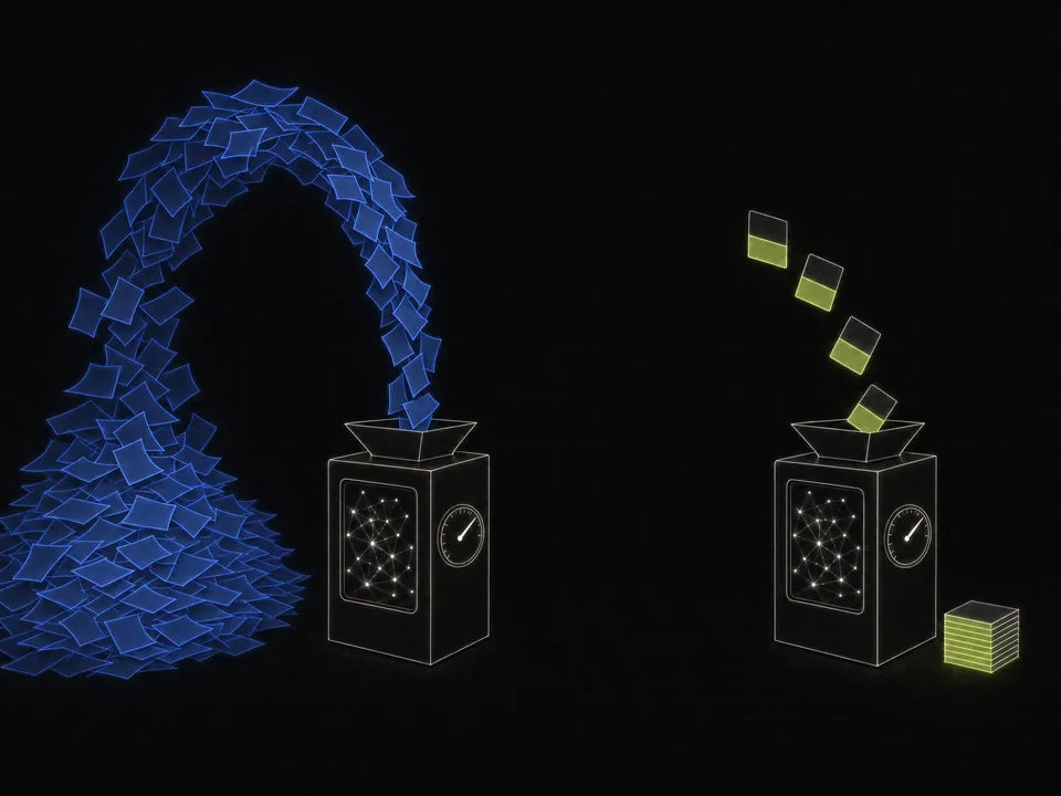 The same network and the same loss. Pretraining feeds it a vast heap of raw text; supervised fine-tuning feeds it a small stack of chosen examples, in which only the answer part is scored.
Two quick checks on telling the stages apart. Pick one option and press Check; a wrong pick shows why it is wrong and keeps the right answer hidden.
A legal-tech startup starts from an open-weight instruction-tuned model. Lawyers write and check 20,000 examples, each a contract clause paired with the structured JSON summary customers want. The team trains the model to produce the JSON given the clause, with the usual next-token loss on the JSON. Which stage is this?
Choose one answer, then check.
A team shows raters two responses to the same prompt and records which one they prefer. It then trains the model directly on these (prompt, preferred, rejected) triples with a loss that raises the preferred response's probability relative to the rejected one. No separate scoring model is trained. Which method is this?
Choose one answer, then check.
Why a company would do only post-training
Start with cost. Training compute grows with the number of parameters times the number of training tokens. A widely used estimate, which you will derive in module 9, is about 6 operations (multiplications and additions) per parameter per token: 2 for the forward pass, which computes the predictions (the multiply and add per parameter you met above), and roughly 4 for the backward pass, which computes the gradients that gradient descent follows. Write for the number of parameters and for the number of training tokens. For a 70-billion-parameter model pretrained on 15 trillion tokens,
Suppose each GPU sustains operations per second, roughly the right order of magnitude for current data-center GPUs running well. The run then needs GPU-seconds. A day has 86,400 seconds, so that is about 182,000 GPU-days: around 18 days on 10,000 GPUs, before counting failed experiments, restarts and the data work.
Now fine-tune the same model for one pass over 100,000 demonstrations of about 1,000 tokens each, which is tokens:
At the same speed that is GPU-seconds, about 29 GPU-hours, or under four hours on one machine with 8 GPUs. Divide the two estimates and cancels, because the model is the same: the ratio is . For the same model, the compute ratio is just the token ratio.
These are idealized estimates. Real runs waste some compute, and reinforcement-learning stages, which generate many long attempts, can cost far more than supervised fine-tuning. For adapting an existing model, the gap is still enormous.
Try the same comparison with a smaller model. The answer box reads scientific notation: 2.4e8 means .
An 8-billion-parameter model was pretrained on 12 trillion tokens. You fine-tune the same model for one pass over 300,000 conversations that average 800 tokens each. Using the estimate ( parameters, training tokens), how many times more compute did pretraining use than your fine-tuning run? Enter the ratio as a number; scientific notation such as 1.5e5 is accepted.
Type a number: 0.25, -2, 3/4 and sqrt(2) all work. Enter checks.
Cost is the first reason. The others:
- Strong base models are available. Several organizations publish capable open-weight models, so a small team can start from a model whose pretraining already cost millions of dollars of compute.
- Most product value is in the adaptation. A customer rarely needs a model that knows more about the world. They need one that does their task, in their format, within their rules, reliably and cheaply.
A post-training company sells some mix of domain adaptation (contracts in a firm's house style, support answered in a company's voice), format and tool use (reliable JSON, correct calls to a customer's APIs), behavior (tone, refusal policy, safety settings), and smaller, cheaper models made by distillation, together with the evaluations that show whether a change helped.
Post-training has limits. It mostly reshapes what the base model already knows how to do. Teaching it large amounts of genuinely new knowledge through fine-tuning is less reliable, which is one reason products often pair a model with retrieval of documents at question time. And fine-tuning too hard on narrow data can erode general abilities, an effect called catastrophic forgetting, which you measure on your own fine-tuned model in module 9.
Now answer the opening question in your own words. Write a few sentences (at least 60 characters), press Compare with the rubric, and grade yourself against its points.
A company says it "does post-training, not pretraining." In a short paragraph that someone outside machine learning could follow, explain what post-training is, what such a company most likely starts from, and why it would not pretrain its own model.
Saved in this browser as you type.
Where older ideas fit
Most of the ideas inside language models were worked out in older architectures, and one of them is the best place to learn how training really behaves.
Convolutional networks (CNNs) handle images by sliding one small grid of weights, a kernel, across the whole image. The same weights are reused at every position: weight sharing across space. A pattern detector learned in one corner then works everywhere, and far fewer parameters are needed. Connecting every value of a 224 by 224 color image ( numbers) to just 1,000 units takes weights. Sixty-four different 3 by 3 kernels over the 3 color channels take .
Recurrent networks (RNNs) handle sequences by reading one token at a time and carrying a hidden state, a vector that summarizes what has been read so far. The same weights process every step: weight sharing across time. Plain RNNs struggle to use information from far back, because the training signal is multiplied by a similar factor at every step it travels back, so it shrinks or explodes geometrically. LSTMs add a gated memory cell that lets information, and the training signal, pass through many steps nearly unchanged. From roughly 2014 to 2017 they were the default choice for sequence tasks such as machine translation, speech recognition and language modeling.
Transformers (2017) replaced recurrence with attention: every position computes dot-product scores against the other positions and takes a weighted average of what it finds. No information has to survive a long chain of steps, and all positions of a training sequence can be processed in parallel, which suits GPUs far better than a step-by-step loop. The price is that attention's cost grows with the square of the sequence length.
So why spend two modules on recurrent networks and LSTMs?
- They show why deep networks are hard to train. The vanishing and exploding gradient story runs from eigenvalues in module 4 through vanishing gradients in RNNs to why the LSTM's gradients survive. The same reasoning explains why transformers are built around residual connections, which add each block's output to its input.
- Gating comes back. The LSTM multiplies a signal, entry by entry, by a learned factor that depends on the input, so the network decides how much passes. The same trick appears in the gated feed-forward blocks (such as SwiGLU) of many current transformers.
- You can own one completely. An LSTM is small enough to design by hand, train in your browser and inspect cell by cell, which is module 8.
One question on the section's main point: what attention gained over recurrence.
Which is the best summary of why transformers replaced LSTMs as the architecture for large language models?
Choose one answer, then check.
Finding objects in images
You may have met R-CNN years ago and wondered why it needed so many versions. The whole family is one idea applied again and again: stop recomputing what can be shared.
The task is object detection: draw a box around each object in an image and name it. The naive approach is to slide a classifier over every window, at every position, size and shape, and run a CNN on each. Count the windows. A 64 by 64 window moved 8 pixels at a time across a 640 by 480 image fits at horizontal positions and vertical ones, so windows, for a single window size and shape. Every extra size or aspect ratio adds thousands more, each needing a full CNN run.
- R-CNN (2014) used a classical, hand-designed algorithm (selective search) to propose about 2,000 regions likely to contain an object, warped each to a fixed size, and ran the CNN on each one separately: still about 2,000 CNN runs per image.
- Fast R-CNN (2015) ran the convolutional layers once on the whole image to get a feature map, a grid of learned features, then pooled each proposed region's part of that map to a fixed size (RoI pooling, for region of interest) and classified it with a few small layers. The expensive computation became shared.
- Faster R-CNN (2015) learned the proposals too, with a small region proposal network on the same feature map.
- Mask R-CNN (2017) added a small branch that predicts a pixel mask for each detected object: instance segmentation, which separates one person from the person standing next to them.
- Fully convolutional networks (FCN) and U-Net (2015) label every pixel in one pass, with no proposals: semantic segmentation. U-Net, designed for biomedical images, shrinks the image and expands it again, with skip connections joining the two paths.
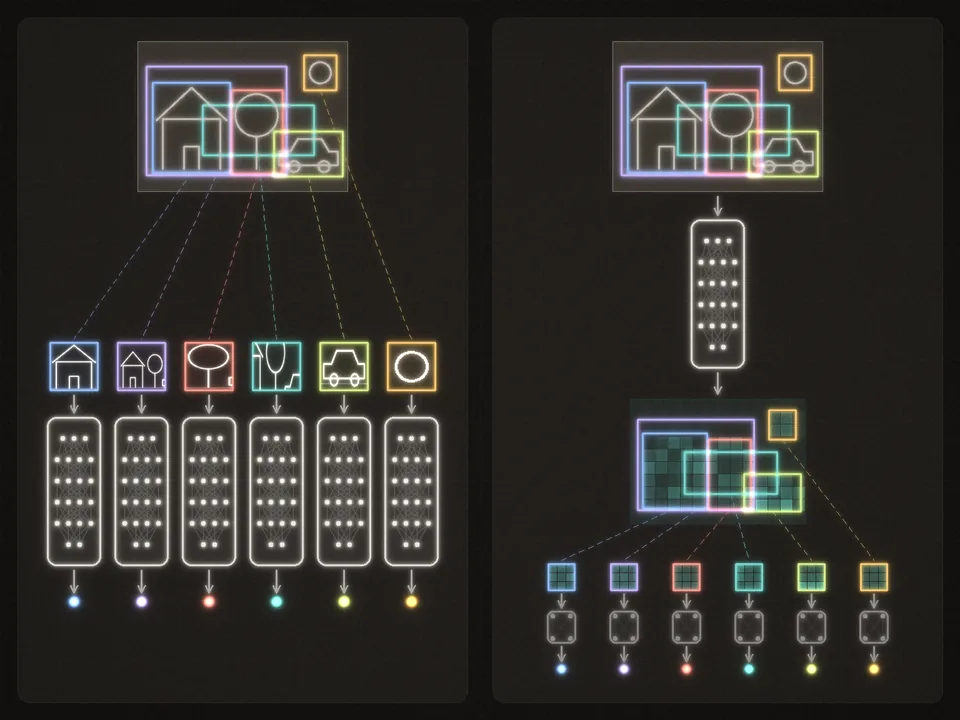 R-CNN runs the expensive network once for every proposed region. Fast R-CNN runs it once for the whole image and cuts each region out of the shared feature map.
| Method | Expensive network runs per image | What changed |
|---|---|---|
| Sliding windows | thousands for each window size and shape | nothing shared |
| R-CNN | about 2,000 | classify proposed regions only |
| Fast R-CNN | 1, plus a few layers per region | share one feature map |
| Faster R-CNN | 1, plus small proposal and head networks | learn the proposals on that map |
| FCN, U-Net | 1 | label every pixel directly |
Module 9 treats convolution and this progression properly, with an interactive comparison, and Part 5 of the roadmap is devoted to vision.
Now count windows yourself, and enter the count as a whole number.
An image is 400 pixels wide and 300 pixels tall. A 50 by 50 window slides across it 10 pixels at a time, horizontally and vertically, and never hangs off the edge. How many window positions are there? A sliding-window detector would run its CNN once at each one. Enter a whole number.
Type a number: 0.25, -2, 3/4 and sqrt(2) all work. Enter checks.
The map of this course
Part 1 rebuilds the math first and then the machine, and each module feeds a later one.
If you keep one thread in mind, keep this one: the eigenvalues of module 4 decide whether gradients vanish or explode in module 7, and the LSTM's cell state in module 8 is the fix. Next, a short tour of how this lab works, with your first Python.