
Lesson 2 of 5
Predicting the next character
A character language model turns every hidden state into a probability for each possible next character, and it is trained to make the real text probable. The loss is the average cross-entropy, the same objective used to pretrain GPT-style models.
Write the loss of a character language model and show that it is the negative log-probability of the text, per character.
Read any loss as a perplexity, the number of equally likely choices it corresponds to.
Build a vocabulary, encode text as ids, and cut training windows whose targets are the inputs shifted by one.
Explain teacher forcing and why one forward pass over a window gives a prediction at every position.
Compute honest baselines (uniform, unigram and bigram cross-entropy) that a trained model has to beat.

Read this and say what comes next: "to be, or not to b". Almost certainly "e". Now this: "First Citizen:" followed by a newline. Here many characters are possible, although a capital letter is likely. A language model is a machine that answers "what comes next" with probabilities: a number for every possible next character, adding up to 1.
That is all a language model is, and it is also what the largest models do. The big picture described a language model as a function from a sequence to a probability distribution over the next token. This lesson makes that concrete with the RNN from the previous lesson. We turn its outputs into probabilities, define the loss, prepare the Shakespeare text as training data, and measure the baselines a real model has to beat. Writing text with the model is the next lesson, and training it is the one after, backpropagation through time.
A probability for every next character
The RNN gives us a state after every character. A language model needs probabilities, so the first job is to turn a state into a probability for each possible next character.
At step the RNN has read the characters up to and including (the -th character of the text) and holds the state . Its output layer produces one score, a logit, for each of the characters in the vocabulary, and a softmax turns the scores into probabilities:
Here is entry of , and is the model's probability that the next character, , is character . Each is positive, and dividing by their sum makes them add up to 1. The softmax, its numerically stable form and its gradient are the subject of softmax and cross-entropy in module 6; nothing about them changes here.
The loss at step is the cross-entropy with the character that actually came next: the negative log of the probability the model gave it. Writing for the id of , the target at step ,
If the model gave the right character probability 1, . If it gave it 0.01, . The loss is the average over all predictions in the text. Its unit is the nat (because the log is natural); divide by to get bits.
A worked example. After "to b", suppose the model gives five candidates the logits for (e, a, o, i, y); a real model scores all 60 characters, but five keep the arithmetic short. Exponentiate each logit:
They add up to . Dividing each by that sum (for e, ) gives the probabilities for (e, a, o, i, y). The target is e, so the loss is .
The instrument below holds exactly this prediction. The blue bars at the top are the five logits; the white bars under them are the probabilities; the dashed lime box marks the target, e; the amber bars at the bottom are the gradient of the loss with respect to each logit, , where is the one-hot vector of the target. The readouts give the loss and .
The loss of a whole text
One position gives one loss. A text gives a prediction at every position, and the loss averages them. Why this score, the average of , and not some other way of combining the predictions? This section answers that, first with numbers and then in general: it is the one that measures how probable the model finds the whole text.
The diagram below computes the loss of the text "hello" from start to finish. It uses a made-up table of probabilities (a real model would compute each row with the softmax above), so every number can be checked by hand.
Why the average of logs is the right loss
Step 5 of the diagram found that the sum of the four losses is , and that is the probability of the whole continuation. That is not a coincidence, and it is the reason for this loss.
Probability has a chain rule: the probability of a whole sequence is the product of each element's probability given everything before it. For "hello", after the first character h:
The same holds for any text. Write for the probabilities the model assigns. Its is exactly its probability for the next character given all of , because the state has read every one of them. So
where means "multiply together", the way means "add together". Now rewrite the loss one move at a time:
Here is the probability of everything after the first character. Lowering the average loss is exactly raising the probability the model assigns to the training text. Nothing else is being optimized. Everything the model ends up knowing about spelling, words, grammar and who speaks when, it learns because that knowledge makes the real next character more probable.
The log also explains step 4 of the diagram. A probability of 0.25 on the truth costs , while raising a good prediction from 0.8 to 0.9 saves only . The log punishes a low probability on the truth far more than it rewards a high one, so the cheapest way to lower the loss is to stop being confidently wrong.
Perplexity
A loss of 0.6020 nats is hard to picture. Perplexity turns a loss back into something you can:
Start with a model that spreads its probability evenly over characters. Every prediction costs , so its loss is and its perplexity is . Reading that backwards: a perplexity of says that, on average, the model is as uncertain as if it were choosing uniformly among characters. For "hello", : the model does about as well as one choosing uniformly among 1.8 characters at every step.
There is a second way to see the same number. Put into the exponent and use :
the -th root of . For "hello" that is , and the fourth root of is : the geometric mean of the four inverse probabilities , , and .
To recap this section: a text's loss is the average of (probability of the true next character); that average is ; and reads it as an effective number of choices.
Now do the whole computation yourself on a three-character text: the losses, the product, the perplexity, and a uniform model for comparison.
A language model reads "the " (with a trailing space) one character at a time. After "t" it gives the next character "h" probability 0.4, after "th" it gives "e" probability 0.8, and after "the" it gives the space probability 0.5.
- Compute the three losses and their average, .
- Check that the sum of the losses equals of the product of the three probabilities.
- Compute the perplexity and say in words what it means.
- A uniform model over 27 characters (26 letters and a space) gives every character probability . What are its loss and its perplexity?
To check your work, enter two numbers as a column: from part 1 (4 decimals), then the perplexity from part 3 (3 decimals).
Work it on real paper: writing each step is the point. Then check your final answer here and compare your working with the walk-through.
One entry per box, top to bottom. 0.25, -2, 3/4 and sqrt(2) all work. Enter moves to the next empty box and checks once all are filled.
From text to training pairs
The diagram worked on one five-character word. To train, we need the same inputs and targets for the whole Shakespeare text, in pieces a network can process. The text becomes numbers in three steps.
The vocabulary. Collect the distinct characters and sort them, so the ids do not depend on the order in which characters first appear. Our Shakespeare excerpt has 100,020 characters and 60 distinct ones: newline, space, eight punctuation marks (! ' , - . : ; ?), 24 capital letters (there is no X or Z) and all 26 lowercase letters. Sorting by character code puts newline at id 0 and space at id 1. Two dictionaries go with it: stoi from character to id ("string to integer") and itos back.
Encoding. Replace every character by its id. The whole text becomes one long array of integers from 0 to 59, and decoding reverses it.
Windows and targets. Training uses short windows of the text. A window of length starting at position gives inputs and targets
Python slices include the start and exclude the end, so holds positions to and holds positions to : the targets are the inputs shifted by one character, exactly as in step 2 of the diagram. With the text "First Citizen", and , the inputs are "First" (positions 0 to 4) and the targets are "irst " with a trailing space (positions 1 to 5): after "F" predict "i", after "Fi" predict "r", and so on. One window is training examples, each with a different amount of context, from one character up to . The last target is ids[s + T], so a start is valid only if is still inside the text: a classic off-by-one.
A batch stacks windows from random starts into arrays. We hold out the last 10% of the text (10,002 characters) as a validation set and train on the first 90,018 characters, so we can tell learning from memorizing.
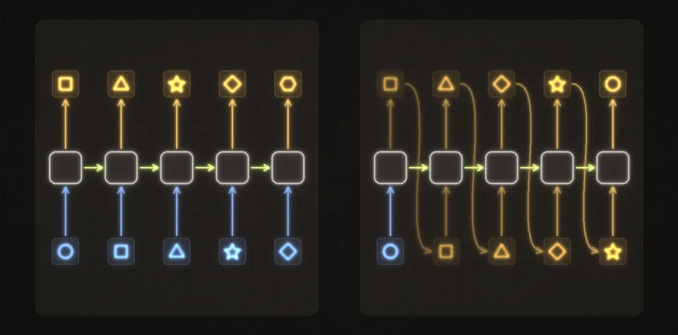 Training reads the true text at every step and checks every prediction at once; generation feeds each chosen character back in, one at a time.
Run this to see the data. It builds the vocabulary, counts the characters and cuts three random windows.
In every printed pair the second string is the first moved one character to the left, with one new character at the end. Check that you can cut a window by hand, including the last valid start.
The text is "to be or": 8 characters at positions 0 to 7. You cut a training window of length starting at position . What are the inputs X and the targets Y?
Choose one answer, then check.
Now write the pipeline in code: the vocabulary, encoding and decoding, and the windows with their shifted targets, including the off-by-one check at the end of the text.
Turn the Shakespeare text into training data.
build_vocab(text)returns the sorted distinct characters and the two lookup tables.encode(s, stoi)anddecode(ids, itos)convert between strings and integer arrays.encoderaisesValueErrorfor a character that is not in the vocabulary.make_windows(ids, seq_len, starts)cuts one window per start, with the targets shifted by one, and raisesValueErrorfor a start that is negative or would need a target past the end of the text.
raise NotImplementedError, then press Run tests. Each check says what it expects.Baselines: how good is good
A loss number means little on its own. Is 2.5 good? Before training anything, compute what simple models score on the same validation text. A trained RNN has to beat all of them, or it has learned nothing worth its parameters.
Uniform. Give every character probability . Every prediction costs , so and the perplexity is 60. An untrained network with small random weights produces nearly equal logits, so its loss starts close to this value. That is the sanity check from module 6: at step 0, expect .
Unigram. Ignore the context and predict each character with its overall frequency in the training text, , where is the number of training characters. Space is the most common character (14,710 of the 100,020 in the whole text, about 14.7%), then "e" (8,900). On the validation text this model scores , a perplexity of about 27.7. (The exercise below adds 1 to every count before dividing, the smoothing explained next; with 90,018 training characters that changes only the fourth decimal.) Knowing that spaces and vowels are common is worth nats per character.
Bigram. Predict each character from the one before it:
where is how often directly follows in the training text, is how often is followed by anything, and is a small smoothing count added to every pair.
A tiny example makes the formula concrete. Take the five-character "text" a b a b b, whose vocabulary has only the two characters a and b, so , and take . Its adjacent pairs are ab, ba, ab, bb. The character a is followed by something twice, both times by b, so , and :
The pair aa never occurs, yet it gets probability , not 0. That is what smoothing is for. Without it, any pair that happens never to occur in the training text gets probability 0, and a single such pair in the validation text makes the loss infinite, because . Our validation text has 12 places where that happens (11 different pairs, such as "Ke" and "xs").
With (add-one smoothing) the bigram model scores on validation, a perplexity of about 10.8.
| model | context used | validation loss | perplexity |
|---|---|---|---|
| uniform | none | 4.094 | 60 |
| unigram | none | 3.323 | 27.7 |
| bigram | 1 character | 2.382 | 10.8 |
A bigram model is the simplest language model with a state: its state is the previous character, and its "weights" are a table of probabilities. An RNN replaces that state with a learned vector that can summarize everything it has read. To show that it uses more than the last character, it has to get below 2.38. The one you train in backpropagation through time does.
The uniform baseline is the one you will use most, as the sanity check for every freshly initialized model. Compute it for a different vocabulary size.
A character model over a vocabulary of 65 characters has just been initialized, and its logits are nearly all equal. What loss should it report on its first training batch? Give 3 decimal places.
Type a number: 0.25, -2, 3/4 and sqrt(2) all work. Enter checks.
Then compute the other two baselines on the real text. Counting is all the training these models need.
Compute the lesson's baselines on the Shakespeare text.
unigram_probs(ids, V, alpha)andbigram_probs(ids, V, alpha): probabilities from counts, with add-alpha smoothing.unigram_loss(p, ids)andbigram_loss(P, ids): the average cross-entropy of predicting every character after the first.
The code at the bottom trains on the first 90% of the text and prints the three validation losses. You should see about 4.094, 3.323 and 2.382.
raise NotImplementedError, then press Run tests. Each check says what it expects.To recap the lesson: the model outputs a softmax over the next character at every position; the loss is the average probability of the true next character, which is ; training windows pair each input with the character after it; and a loss means something only against baselines on the same text. The next lesson uses the model's probabilities for the other half of the job: writing text. First, explain the objective in plain words.
A client asks what "next-token prediction" has to do with how a large language model learns. Using the character model of this lesson, explain what the model outputs at each position, what the loss measures and why minimizing it makes the training text probable, and what a loss number can and cannot tell them.
Saved in this browser as you type.