
Lesson 1 of 5
Attention
Attention lets every position look directly at every other position. Score with dot products, turn the scores into weights with a softmax, and average the values. It is the operation that replaced recurrence and the core of every transformer.
Compute attention scores, weights and the output by hand for one query and a few keys.
Derive why dot-product scores are divided by .
Write self-attention in matrix form with its shapes, and follow every matrix of a three-token example.
Say what queries, keys and values are each for, and why a language model needs the causal mask.
Implement scaled dot-product attention and causal self-attention in numpy.
Explain why attention replaced recurrence, and what it costs.

It is 2014 and you are translating with LSTMs. An encoder LSTM reads the English sentence one word at a time. Its final state, a vector of fixed size (say a thousand numbers), goes to a decoder LSTM, which writes the French sentence from that vector alone. Every word, its order and its role in the sentence has to fit into those thousand numbers, and has to survive the whole trip through the encoder's steps. Researchers found that such systems got worse as sentences got longer.
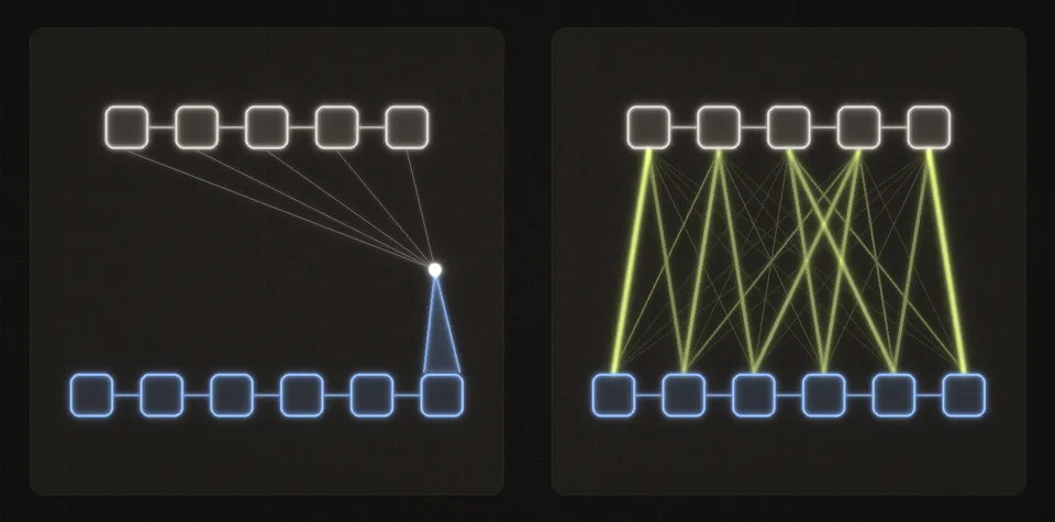 Left: everything the decoder knows must pass through one fixed-size vector. Right: with attention, each output step reaches back to every input, more strongly to the ones that matter now.
The fix is easy to state: let the decoder look back. At each step of writing, it scores every encoder state for how relevant it is to the word it is about to write, and takes a weighted average of them. That is attention. Within three years, a model built from attention alone had replaced the recurrence itself.
This lesson builds attention in four moves. First, one lookup with numbers small enough to check on paper. Second, why the scores are divided by . Third, the same lookup for every token of a sentence at once, drawn matrix by matrix, with what queries, keys and values are each for and the mask that hides the future. Fourth, why this replaced recurrence and what it costs. The next lesson, Inside a transformer, assembles a whole model from it.
A soft dictionary lookup
Attention is a kind of lookup, so start with the most ordinary lookup there is. In Python, prices = {"apple": 3, "pear": 7} and prices["apple"] gives 3. The lookup compares your query, "apple", with every key, finds the one that matches exactly, and returns that key's value.
Attention keeps the three roles and softens the matching:
- A query : what the current position is looking for.
- Keys : what each position offers to be matched against.
- Values : what each position hands over when it is chosen.
All three are vectors, and queries and keys have the same length so that they can be compared. In the translation model, the query is computed from the decoder's current state, and every encoder state supplies one key and one value. The lookup has three steps.
- Score every key by its dot product with the query: . As you saw in module 1, the dot product is large when two vectors point the same way.
- Turn scores into weights with the softmax of module 6: . The weights are positive and add up to 1.
- Average the values with those weights: . The output is what the lookup returns.
One lookup on paper
Here is the smallest example that shows every step. The query is . The keys are , and . The values are plain numbers, , and , so the output is a number too.
Step 1, the scores. Multiply the query and each key entry by entry, then add:
The query points mostly along , so scores highest. It points away from , so scores below zero.
Step 2, the weights. Exponentiate each score. This makes every number positive and keeps their order:
Add them: . Divide each by that sum:
Check: .
Step 3, the output. Multiply each value by its weight and add:
The same computation as one table, laid out the way the widget below lays it out:
| key | score | weight | value | |||
|---|---|---|---|---|---|---|
| sum |
Two things are different from the dictionary. Every key contributes something, in proportion to how well it matches, so the output is a blend that leans toward the best match: 12.92 sits between the three values, closest to . And everything is differentiable. A hard lookup that returns only the best key has zero gradient almost everywhere: nudging the query does not change which key wins, until suddenly it does. The softmax makes every weight a smooth function of the query and the keys, so gradient descent can learn what queries and keys should look like.
Before you try it live, predict what a longer query does. The next question doubles the query and keeps everything else.
In the worked example, the query attends over , and with values , and the output is about . Now double the query to and keep the keys and values. What happens? Decide before you check it in the widget below.
Choose one answer, then check.
The widget below runs the same lookup and answers questions like that one. On the plane, the blue arrow is the query and the three coral arrows are the keys, each tagged with its weight. The values 10, 20 and 30 sit on a number line under the plane as white ticks, and the lime marker on that line is the output . The table under it has the columns of the table above.
Why divide by the square root of d
The widget showed that bigger scores give sharper weights. In real models, queries and keys typically have 64 or 128 entries, not 2, and that alone makes the scores large, for a reason that has nothing to do with how well a key matches. The fix is to divide every score by , where is the length of the query and key vectors:
Here is where the comes from. Suppose the entries of a query and a key behave like independent random numbers with mean 0 and variance 1, which is roughly what careful initialization aims for. (The variance of a random quantity is the average of its squared distance from its mean. Its standard deviation, the square root of the variance, is its typical distance from the mean.) The dot product is a sum of terms, each with mean 0 and variance 1. Its variance is , so its typical size is . For , raw scores have a standard deviation of 8.
Go slower: The variance of a dot product
Assume every and is independent of the others, with and . Here means the average over many random draws, and .
One term, its mean. For independent variables, the average of a product is the product of the averages:
One term, its variance. Use the definition of variance with the mean just found: Squares of independent variables are independent too, so the average of the product splits again:
The sum. The terms are independent of each other, and variances of independent terms add:
The fix. Dividing a random quantity by a constant divides its variance by . With : whatever the dimension.
Why do large scores hurt? Suppose one score is 8 and seven others are 0. The softmax gives the first key : almost all the weight, from a difference that came from the dimension rather than from meaning. Worse, a saturated softmax stops learning. In the Jacobians lesson you derived the softmax's Jacobian, . When is exactly one-hot, say , both and are the matrix with a single 1 in the top-left corner, so their difference is all zeros. When is nearly one-hot, every entry is nearly 0, so almost no gradient flows back into the scores, and the queries and keys that produced them barely change. It is the same saturation you met with sigmoid and tanh.
Run the experiment: 500 random queries, each compared with its own 8 random keys, for three sizes of . The table prints the spread (standard deviation) of the scores before and after dividing by , and the average weight the softmax gives the winning key.
The raw spread grows like : about 2, 8 and 23, against , and . The winning key's average weight climbs from 0.51 to 0.96. After dividing by the spread stays near 1 and the winning weight stays near 0.35 at every size. Softness is not the goal in itself: a trained model can still learn sharp attention by making its queries and keys large along the directions that matter. The division only stops the dimension from deciding that for it.
To recap: a dot product of two random -entry vectors has spread , which would push the softmax toward a single key and stall its gradient. Dividing by brings the spread back to 1. This is scaled dot-product attention, the form the transformer paper introduced and most models since have kept.
The next exercise is one full lookup with , where the division by matters.
With , the query attends over the keys , and , whose values are , and . Compute the scaled dot-product attention output . Enter it as a column, first entry on top, each entry to 2 decimal places.
One entry per box, top to bottom. 0.25, -2, 3/4 and sqrt(2) all work. Enter moves to the next empty box and checks once all are filled.
Every token at once: self-attention
So far one query looked at a list of keys. In a language model, every token of a sentence needs its own lookup: in "the cat sat", the token "sat" should be able to find "cat", and "cat" should be able to find "the". In self-attention, the queries, keys and values all come from the same sequence, so every token is at once a query and a key and value for the others. Done one token at a time this would be slow. Stacked as matrices, all the lookups become three matrix products.
The tokens. Stack the token vectors of a sequence as the rows of a matrix of shape , the row convention from module 2. Row is token 's vector , and is how many numbers each token carries.
Queries, keys and values. Three learned matrices turn every token into its query, key and value:
and have shape and has shape . Row of is , the query of token , and likewise row of is its key and row of its value . Queries and keys have length , which plays the role of from the previous section.
Every score at once. Transposing turns its rows into columns, so column of is the key . Entry of the product is row of times column of , which is . Divide everything by :
is : row holds token 's scores for every token .
Weights and output. A softmax along each row of gives the weight matrix , whose rows each add up to 1. The output is , of shape . Row of is : the lookup from the first section, done for every token in parallel.
The diagram below computes every one of these matrices for three tokens, "the cat sat", with and small whole-number weights, so that every number can be checked by hand. It has eight steps: the formula at the top lights up the part each step computes, the new matrix is drawn in lime, and the text under the figure gives the arithmetic. Step 5 adds a causal mask, which the section after next explains.
To recap: self-attention is the lookup of the first section run for every token at once. holds every score, a row softmax turns each row into weights, and averages the values. For a sequence of tokens, the score matrix alone has entries, which matters at the end of this lesson.
What queries, keys and values are for
Why three learned matrices, rather than one vector per token used for all three jobs? Try the simplest alternative and see what goes wrong. If every token used its own vector as its query, key and value, the score of token for token would be . That is large for tokens whose vectors point the same way as , so every token would mostly look for tokens like itself, and could only hand over its own vector. Separate matrices remove both limits.
The query and the key can differ. A query says what a token is looking for; a key says what a token can be found by. The verb "sat" looks for its subject, while "cat" is not looking for its verb in the same way. With separate and the scores need not be symmetric, and in the diagram they are not: step 3 has but . If the two matrices were equal, every score matrix would be symmetric. Transposing a product reverses the order of the factors and transposes each one, so the raw scores are . With this is , and transposing it by the same rule gives it back unchanged.
The value can differ from the key. Being found and being useful are different jobs. In "the cat that the dog chased sat down", the token "sat" has to find its subject, "cat", by matching on grammatical role, but what it needs to take over is what "cat" means. Separate lets a token be matched on one kind of information and hand over another.
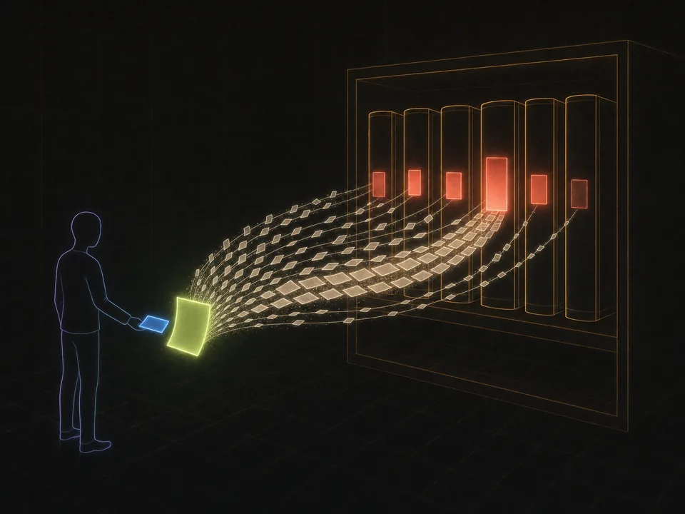 The query is the request, the keys are the labels on the spines, and the values are what the books hand over. Every book contributes, in proportion to how well its label matches.
None of these roles is programmed. , and start random and are learned by gradient descent through the softmax, which is why the smoothness of the soft lookup mattered.
The causal mask
A language model is trained to predict token from tokens to , at every position of a training sequence at once, exactly as your character models were in module 7. If position could attend to position , it could read the answer instead of predicting it. Training loss would fall to nearly zero, and the model would be useless for generation, where the future does not exist yet.
The fix is a mask added to the scores before the softmax:
Any number plus is , and , so blocked positions get weight exactly 0, and each row's softmax spreads its weight over the visible positions only. The full formula becomes .
Go back to steps 5 and 6 of the diagram to see what the mask changes. Without it, the row for "the" would be : the first token would take 67% of its information from "cat", the very word it is trained to predict. With the mask it is . In the same way, "cat" would put 0.576 of its weight on "sat", its own prediction target; with the mask, that weight is 0 and the rest is renormalized to .
The picture below uses the reference implementation in mlref.attention on six random token vectors. The first heatmap has no mask; the second has the causal mask, so everything above the diagonal is 0.
The mask has one more consequence: since token reads only tokens 1 to , its output never changes when later tokens are added. The code exercise below tests exactly that, and the next lesson uses it to make generation fast. First, what happens when the mask is forgotten?
You train a character language model built from self-attention, but you forget the causal mask. Training runs on windows of text with the targets shifted by one, as in module 7. What do you expect?
Choose one answer, then check.
Now put the whole computation together by hand: scaled scores, weights, the output, the causal mask, and what happens without the .
A query attends over three keys in dimensions: , , , , with values , , .
- Compute the scaled scores and the attention weights, to 3 decimal places.
- Compute the output , to 3 decimal places.
- The query now belongs to position 2 of a causal language model, and to position 3, while and belong to positions 1 and 2. Recompute the weights and the output.
- Redo part 1 without dividing by . What changes, and why?
Work it on real paper: writing each step is the point. Then check your final answer here and compare your working with the walk-through.
One entry per box, top to bottom. 0.25, -2, 3/4 and sqrt(2) all work. Enter moves to the next empty box and checks once all are filled.
A few more lookups for practice, each with new numbers:
A query attends over three keys , , , in dimensions. Find the attention weights . Give each to 3 decimal places.
One entry per box, top to bottom. 0.25, -2, 3/4 and sqrt(2) all work. Enter moves to the next empty box and checks once all are filled.
Then build it in code. The exercise checks your attention against the reference, reproduces the diagram's weights for "the cat sat", and tests causality directly: changing later tokens must not change earlier outputs.
Implement attention in numpy, one sequence at a time (no batch dimension), with rows as tokens.
causal_mask(T): a boolean array,Truewhere a query may not look, which is strictly above the diagonal.attention(Q, K, V, mask=None): scaled dot-product attention. Blocked scores become-np.inf, and the softmax subtracts each row's maximum before exponentiating. Return the output and the weights, in that order.self_attention(X, Wq, Wk, Wv, causal=True): project the tokens to queries, keys and values, then attend, with the causal mask whencausalis true.
The tests compare with the reference mlref.attention, reproduce the diagram's weights for "the cat sat", check that the mask gives later positions exactly zero weight, and check causality directly: changing later tokens must not change earlier outputs. The next lesson builds several heads and a whole block on top of this.
raise NotImplementedError, then press Run tests. Each check says what it expects.A transformer layer runs several of these attentions side by side, each with its own , and , so that different heads can look for different things. That, and everything else around attention, is the next lesson.
Why attention replaced recurrence
Attention entered in 2014 as a helper for recurrent networks. In 2017 the transformer dropped the recurrence and kept only attention, and within a few years it had replaced recurrent networks for most sequence tasks. Three facts explain why, and the third is the price.
Short paths. In a recurrent network, information from position reaches position only through steps, and the gradient that trains the connection is a product of Jacobians. As you derived in backpropagation through time, such a product shrinks or grows geometrically, governed by the eigenvalues and singular values of module 4. In self-attention, position reads position directly, in one layer, whatever the distance. There is no long product to vanish.
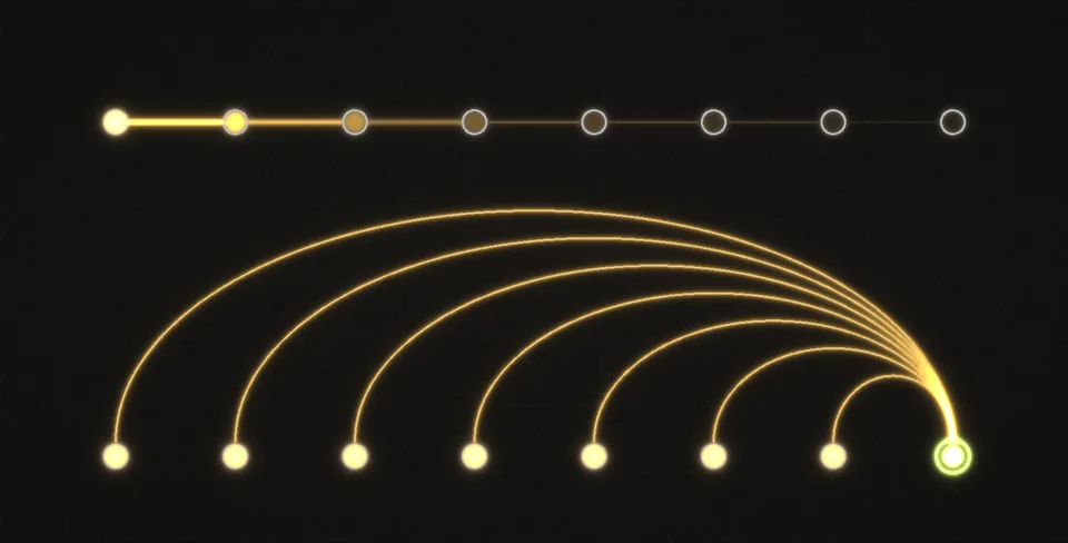 A recurrent network passes information link by link, and the signal weakens at every hop. Attention connects the last position to every earlier one in a single step.
Parallel training. A recurrent network must compute before , and before . A transformer computes every position of a training sequence at once, with a few large matrix multiplications, which is exactly the work GPUs are built for. The causal mask is what makes this legal for next-token prediction.
The cost. Using the cost rule from module 2, takes multiply-adds and takes . The score matrix has entries per head per layer, so doubling the context quadruples that work and memory. For and 32 heads, a single layer computes scores. A recurrent network's cost per step does not depend on how much it has read, and it carries a fixed-size state, while a transformer that generates text must keep something for every earlier token (the next lesson shows what).
To recap: attention replaced recurrence because every position reaches every other in one step and a whole sequence trains in parallel. It pays with a cost that grows with the square of the sequence length. Much engineering goes into that trade: attention kernels that never store the full score matrix at once, and a revival of recurrent and state-space designs, often gated, that carry a fixed-size state again.
The last exercise asks you to put this argument in your own words, for someone who knows recurrent networks well.
A colleague who trained LSTMs years ago asks why transformers replaced them. Explain the two main reasons and what attention costs in exchange, using what you know from modules 4 and 7 about long products of Jacobians. Then say honestly what recurrent designs still offer.
Saved in this browser as you type.