
Lesson 2 of 2
How this lab works
How each kind of exercise works and how to use it honestly, Python and numpy running in your browser, the numpy that the rest of Part 1 needs, and a way of studying that makes the material stick.
Use each exercise type as it is meant to be used, from paper derivations to code that must pass tests.
Run Python in the browser, print numpy arrays and draw a live chart with
show.line.Compute a mean, variance and standard deviation by hand, with loops, and with numpy.
Predict the shape of a numpy result after indexing, an
axisreduction, broadcasting or@.

This lab is built for doing, not only reading. Most pages ask you to work something out on paper, type an answer that gets checked, or write a function that has to pass tests. That is deliberate: reading a derivation feels like understanding it, and the feeling is often wrong until you try to reproduce it.
This lesson shows each kind of exercise at the moment you first meet it, gets Python running in your browser, and covers the numpy you need for the rest of Part 1. Along the way you will write, in a few lines of numpy, the arithmetic of layer normalization, one of the steps inside a transformer block.
Exercises you check yourself
Every exercise sits on a card, and a label at the top of the card says its kind:
- On paper. A calculation or derivation you work with pencil and paper, then check and compare step by step.
- Work it out. A typed answer (a number, a vector or a matrix), checked as soon as you submit it.
- Quick check. Multiple choice, with a note on every option.
- In your own words. A short written explanation that you compare with a rubric.
- Code it. Python with numpy, graded by tests.
- Practice set. Fresh problems from a generator, as many as you want.
Each kind is explained where it first appears in this lesson: paper and typed answers in this section, code in the next two, quick checks in the second numpy section, and the rest near the end. When you finish a card, a tick and a word such as Correct or Passing appear in its header.
The math for the first exercises
The first exercises use three statistics that come back in the numpy sections. For a list of numbers :
- The mean is the average, . The Greek letter (mu) is the usual name, and means "add up the following for ".
- The variance is the average squared distance from the mean, . Squaring makes every distance count as positive, so points below the mean cannot cancel points above it.
- The standard deviation is its square root, (sigma). It measures spread in the same units as the data.
A worked example with . The mean is . The distances from the mean are , , and . Their squares are , which add to . So and . In an answer box you could type that last answer as sqrt(5).
How a paper exercise works
A paper card has the question, answer boxes with a label that lists what goes in them, and a button that opens the worked steps. Work through it in this order:
- Solve the whole problem on real paper before touching the card. Writing each step is the point.
- Type your final numbers into the boxes, in the order the label lists them (a column of boxes is filled top to bottom), and press Check. Enter works too: it moves to the next empty box, and checks once every box is filled. The card then says "Your final answer matches", or says which answers do not match yet and highlights their boxes.
- Press "I have my answer. Walk me through it." The first step of the worked solution appears. Press "Next step (2 of 5)" to reveal one more, or "Show all steps".
- Compare line by line. If your answer did not match, stop at the first step where your working differs, and redo the rest yourself before revealing more.
- Grade yourself. After the last step comes a summary and the question "How did your working compare?", with Got it, Partly and Missed it. Partly or Missed it puts the exercise on the review list of the Practice page until you mark it Got it, so be honest.
Many cards also have hints, behind a link such as "Show hint 1 of 3". They open one at a time, from a nudge to most of the first step. Try this one on eight numbers:
Take .
- Compute the mean , the variance (divide by ) and the standard deviation . Write every distance from the mean before squaring.
- Without recomputing from scratch, say what happens to all three if you add 10 to every number, and if instead you multiply every number by 3.
Enter your three answers to part 1 top to bottom: the mean, the variance, then the standard deviation. Part 2 has no box: compare it with the walk-through.
Work it on real paper: writing each step is the point. Then check your final answer here and compare your working with the walk-through.
One entry per box, top to bottom. 0.25, -2, 3/4 and sqrt(2) all work. Enter moves to the next empty box and checks once all are filled.
Typed answers
A Work it out card has one box for a number, a column of boxes for a vector (entered top to bottom), or a grid for a matrix (entered row by row). You can type:
- plain numbers, such as
0.25,-2or1.5e13(scientific notation: ); - exact expressions, which the checker evaluates:
3/4,sqrt(2)/2,2^10,pi,e,ln(2), and arithmetic such as(2 + 4)/3.
Press Check, or Enter. An answer passes when it is close enough. Unless the question asks for a number of decimal places, the allowance is 0.01 or half a percent of the answer, whichever is larger, which forgives rounding to two decimal places. When a question asks for 3 decimal places, give 3: an answer rounded further gets "Close, but rounded too far" and does not pass.
A wrong answer turns its box red and says "Not yet. Check your arithmetic and try again"; for a vector or matrix, only the entries that are off are highlighted. After a second miss, the message points you to the hints and the worked solution. An empty box, or text that is not a number, gets a message instead of a verdict and does not count as a try. The worked solution sits behind a link at the bottom of the card. Before your first try, that link pauses to ask "Struggling first is where the learning happens. Still show it?", with Show it and Keep trying.
Practice the exact form once. The standard deviation below is a square root, so type it as an expression rather than a rounded decimal.
What is the standard deviation (divide by ) of ? Give it exactly, as an expression of the form sqrt(a)/b or sqrt(c) with your own numbers, or as a decimal to 3 decimal places.
Type a number: 0.25, -2, 3/4 and sqrt(2) all work. Enter checks.
Python in your browser
Code exercises need Python, and here it runs inside your browser tab. Python 3.14 and numpy are compiled to WebAssembly (the project is called Pyodide) and run in a background worker, so nothing you write is sent to a server. Python starts loading as soon as a code cell comes near the screen. The first time, the browser downloads Python and numpy, about 9 MB; after that they come from the browser's cache and start in a few seconds. The small dot on the right of each code toolbar shows whether Python is idle, loading, ready or running (hover over it to read which).
The cell below is a runnable example, the kind that appears inside lessons. With it:
- Press Run, or put the cursor in the code and press Cmd+Enter on a Mac (Ctrl+Enter on Windows and Linux) or Shift+Enter.
- Edit anything. An Original button appears as soon as you change the code, and brings back the code as written.
- Each run starts from a clean slate: variables from the previous run are gone.
- While code runs, a Stop button appears next to Run. Stop ends the run by restarting Python, which is the way out of an infinite loop or a training run you want to cut short.
For open-ended experiments, the Lab page has a scratchpad where variables persist between runs, like a notebook.
Inside every cell, np (numpy) and math are already imported, along with the course helpers: show.line, show.bars and show.heatmap draw live charts under your code, and expect_close and friends are what the tests use. show.line("loss", value) adds one point to a chart named "loss" each time it is called, so a chart grows while a loop runs. Press Run.
The first three printed lines give the array, its shape (4,), and mean 5.0, variance 5.0 and standard deviation 2.2361, matching the worked example above. The chart named loss has 40 points: it starts at 9, drops fast and flattens near 0, and the last line prints final w = 2.9996.
You can see why from the update line. It subtracts from , so the distance to 3 goes from to : it shrinks by the same factor 0.8 every step, and the loss, its square, by . That is why the chart reads 9, then , then : big steps while far away, tiny steps when close. Every training run in this course ends with a chart like this one, and reading its shape is a skill you will build in module 6.
Your first code exercise
Every module has code exercises, and this first one exists mostly to learn how they work. A code card holds the prompt, a toolbar, an editor with the starter code, and an output area under the editor. The starter defines the functions you must write, with a description of each, numbered comments that outline the steps, and raise NotImplementedError where your code goes. Here is what happens as you work through it:
- Run the starter as it is. Press Run tests (or Cmd+Enter, Ctrl+Enter or Shift+Enter in the editor). An amber note says the code is not finished yet: part of it still says
raise NotImplementedError. Below it comes the summary "0 of 7 checks pass. Each one waits on code you have not written yet." and the list of checks, each marked with an hourglass and "waiting for your code". Each check's name is a requirement, such as "variance([1, 3]) is 1: divide by n, not n - 1". A run like this does not count as an attempt. - Write one function and run again. Checks that now pass get a tick; the amber note stays until no function still says
raise NotImplementedError. A check that fails gets a cross and a message saying what it expected and what your code produced, for example "variance([2, 4, 4, 4, 5, 5, 7, 9]) should be 4, but it is 4.57143." (that variance divided by ). A check whose code crashed gets a warning triangle and the error. The summary line counts the checks that pass; start with the first one that did not. - If your code stops at an error before the checks run, the output says so and shows the line and the error message. Fix that line and run again.
- When every check passes, the output reads "All 7 checks pass. This exercise now counts as passing." and the card is marked Passing.
- Your draft is saved in this browser as you type. Reset to starter puts the starter back, and Bring back my code undoes that. The Reference solution link at the bottom asks you to run your own code first; after a real attempt it opens straight away, with a button that puts the solution in the editor, which you can also undo.
The statistics from the paper exercise, now as code:
Write mean(xs), variance(xs) and std(xs) for a Python list of numbers using plain loops, no numpy inside them. Use the definitions from the lesson: divide by , not . mean should raise ValueError for an empty list. Run the starter first to see what unfinished code looks like, then fill it in one function at a time.
raise NotImplementedError, then press Run tests. Each check says what it expects.Arrays, shapes and axes
Loops over Python lists are fine for ten numbers and hopeless for ten million. numpy stores numbers in compact arrays and runs whole-array operations in compiled code. Part 1 needs only a handful of its ideas, in two groups: this section covers arrays, shapes and sums along an axis, and the next covers broadcasting and matrix products.
Arrays and shapes. np.array([[1, 2], [3, 4], [5, 6]]) makes a two-dimensional array with 3 rows and 2 columns. Its shape is (3, 2): rows first, then columns. In code, this course stores a batch as an array X of shape (n, d): one row per example, one column per feature. (Math writes a single vector as a column; module 2 explains why code uses rows for batches.)
Indexing. Positions count from 0. X[1] is row 1, the second row. X[:, 0] is column 0 (the colon means "every row"). X[2, 1] is a single entry: row 2, column 1. X[-1] is the last row, and X[0:2] is rows 0 and 1 (the end of a slice is excluded).
Elementwise arithmetic. +, -, *, / and functions such as np.exp and np.sqrt act on each entry separately. X * X squares every entry; it is not matrix multiplication.
Reductions along an axis. A reduction turns many numbers into one, the way a sum or a mean does. X.sum() adds every entry. X.sum(axis=0) adds down the rows, collapsing axis 0, so one number remains per column. X.sum(axis=1) adds across each row, so one number remains per row. The same goes for mean, std, max and argmax (the position of the largest entry). With the 3 by 2 array above:
The rule to remember: the axis you name is the one that disappears from the shape. has shape (3, 2). Summing over axis 0 removes the 3 and leaves shape (2,); summing over axis 1 removes the 2 and leaves shape (3,).
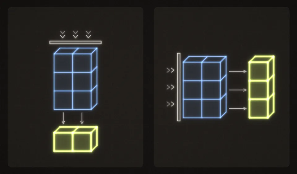 The axis you name is the one that disappears. Axis 0 collapses the rows and leaves one number per column; axis 1 collapses the columns and leaves one number per row.
Check the rule on a new array. This is a vector answer: one box per entry, top to bottom.
X = np.array([[2, 0, 1], [1, 3, 5]]). What is X.sum(axis=0)? Enter it as a column, first entry at the top.
One entry per box, top to bottom. 0.25, -2, 3/4 and sqrt(2) all work. Enter moves to the next empty box and checks once all are filled.
Broadcasting and matrix products
Real code combines arrays of different shapes all the time: subtracting a mean from every row, adding a bias to every example. numpy's rule for this is called broadcasting, and it is the source of the quietest bugs.
Broadcasting. When two arrays have different shapes, numpy compares the shapes from the right. Two sizes are compatible if they are equal or if one of them is 1, and a size of 1 (or a missing dimension) is stretched to match. So X - X.mean(axis=0) subtracts the column means (3, 4), shape (2,), from every row of the (3, 2) array:
Row means have shape (3,), which does not line up with (3, 2) from the right: 3 against 2. Asking for X.mean(axis=1, keepdims=True) keeps the collapsed axis as size 1, giving shape (3, 1), which stretches across the columns. Module 2 draws these rules with pictures.
Matrix multiplication. A @ B multiplies matrices. A shape (n, d) array times a shape (d, k) array gives shape (n, k): the inner sizes must match, and they disappear. X @ w with w of shape (d,) gives shape (n,), one number per row, each the dot product of that row with w: multiply matching entries and add. So that single line computes one neuron's weighted sum for every example in the batch at once, and with a matrix W of shape (d, k) in place of w it computes a whole layer of neurons. Module 2 and module 6 build on exactly this.
Random numbers. rng = np.random.default_rng(0) creates a random generator with seed 0. rng.normal(size=(2, 3)) draws a 2 by 3 array of normally distributed numbers, and rng.integers(0, 10, size=5) draws whole numbers from 0 to 9. The same seed gives the same numbers every run, which is how tests stay repeatable.
Run the tour, then change things: other axes, other shapes, a deliberate mismatch.
Read the output against the text. X @ w is [ 8 26 44], because each row is dotted with : , and . The (3, 2) @ (2, 4) product has shape (3, 4). The heatmap shows the 4 by 6 random scores, and argmax(axis=1) picks the column of the largest score in each row, [2 0 1 3] with seed 0. The last line is numpy refusing to combine shapes (3,2) and (3,).
The next card is a quick check. Pick an option and press Check. If your pick is wrong, it is marked, the note under it says why, and the right answer stays hidden so that your next try is real; Check stays greyed out until you change your pick. When you are right, every option shows its note. Read the notes on the wrong options too: they are the mistakes people actually make. Some quick checks ask you to choose every option that applies, and the card says so above the options.
X holds a batch of token vectors with shape (32, 10): 32 rows, one per token, and 10 features each. Which line standardizes each row on its own, so every row ends with mean 0 and standard deviation 1?
Choose one answer, then check.
Now put it together. In the next exercise you standardize a batch two ways: each column (feature) across the batch, and each row (example) on its own. The second is exactly the arithmetic of layer normalization. The tests use a batch that is not square, then one that is, where the wrong axis would run without an error.
X is a batch with shape (n, d): one row per example, one column per feature. Using numpy and no Python loops, write:
column_stats(X): the mean and standard deviation of each column, each of shape(d,).standardize_columns(X): every column rescaled to mean 0 and standard deviation 1.normalize_rows(X, eps=1e-5): every row standardized on its own, , where and are that row's mean and variance and (epsilon) is a small constant that keeps a constant row from dividing by zero.
The tests use batches that are not square, then one that is, so the wrong axis cannot hide.
raise NotImplementedError, then press Run tests. Each check says what it expects.Explanations, practice sets and checkpoints
Three more kinds of exercise remain, and each works differently from the ones you have used so far.
In your own words. You met one at the end of the previous lesson. Write in the box as if explaining to a smart friend who has not taken this course. The Compare with the rubric button works once you have written 60 characters. It opens "A strong answer covers", three or four points a good answer makes, and "One way to say it", a model answer. Then grade yourself: Covers them all, Covers some or Missed most. Your text is saved in this browser as you type and is never sent anywhere.
Practice sets. A practice set makes a fresh problem every time from a generator. Type your answer (or pick an option) and press Check or Enter. Right or wrong, the worked solution appears. Then press New problem (or Enter again). The dots at the top count your streak: three right in a row completes the set, and a miss starts the count again. The first one is in Arrows and lists, and the Practice page collects them all.
Checkpoints. At the end of each module, a checkpoint asks 8 to 12 questions in new situations; this module's has 10. Answer all of them, then press Submit checkpoint once. If any are blank or hold something that is not a number, it asks first, with Go to question and Submit anyway, because unanswered questions count as wrong. A code question counts when you have run its tests inside the checkpoint and they pass. After submitting you see your score, each question marked Correct, Not quite or Not answered with its explanation, and links to the ones you missed. You need 80 percent to pass. Retake with blank answers starts again, and after a pass a button leads on to the next module.
How to study here
A few habits make a large difference.
- Paper before steps. Commit to an answer before revealing anything. If your check fails, reveal one step at a time until you find where you split from the worked solution, then redo the problem from that point without looking.
- Hints before solutions. Open hints one at a time. If you open a worked solution before trying, the link asks you to confirm first, because the struggle is where the learning happens.
- Run the starter. A failing check's message is a hint in disguise. Read it before reading the reference solution.
- Use the checkpoint as a gate. Take it at the end of each module and do not move on until you pass. If you miss items, revisit those lessons, then retake it on another day.
- Come back for practice. The Practice page has every practice set, plus a review list of what you have missed so far: typed answers and quick checks not yet answered correctly, and paper exercises you marked Partly or Missed it. A few problems a day beat an hour once a week.
Your progress lives only in this browser. The Progress page keeps separate records for lessons you have marked as read (with the button at the bottom of each lesson), answers that were checked correct, code that passed its tests, and your own self-grades, because these are different kinds of evidence. Export a backup there if you switch devices. A passed checkpoint means you handled that module's questions; it is a record for you, not a certificate of professional skill. The Glossary collects every term in plain words, with a link to where it is taught.
That is the whole lab. Next comes the first real mathematics: vectors and the dot product.