Rank and low-rank updates

Back to the two microphones from the last lesson. In the bad arrangement, microphone 2 hears exactly half as much of each voice as microphone 1:

(The second column is half the first, so $x_2$ copies of it are $\tfrac12 x_2$ copies of the first.) Two voices go in, but every pair of recordings is a multiple of $(2,\allowbreak 1)$: one number's worth of information comes out. And some pairs of voices vanish completely. Voices $(1,\allowbreak -2)$ give recordings $\left(1 + \tfrac12(-2)\right)(2,\allowbreak 1) = 0 \cdot (2,\allowbreak 1) = (0,\allowbreak 0)$.

The determinant said "zero, information is lost". This lesson says how much: one dimension survives, and one is crushed. That count is the rank. Then comes the twist. A matrix that keeps only a few dimensions is also a matrix that takes very few numbers to write down, and that is exactly the idea behind LoRA, one of the most widely used ways to fine-tune large language models cheaply.

#Column space, null space and rank

Some matrices cannot be undone. To say how much they lose, we need names for what they keep and what they crush.

One word first: the dimension of a line, plane or larger flat space through the origin is the number of vectors in a basis for it (module 1): 1 for a line, 2 for a plane, $n$ for all of $\mathbb{R}^n$, the space of lists of $n$ numbers. Every basis of the same space has the same number of vectors, so the dimension is well defined. Now three definitions, each shown on the bad microphone matrix.

• The column space of $\mathbf{A}$ is the set of all outputs $\mathbf{A}\mathbf{x}$. Since every output is a combination of the columns, it is the span of the columns (module 1). For the microphones: every multiple of $(2,\allowbreak 1)$, a line.
• The null space of $\mathbf{A}$ is the set of all inputs that $\mathbf{A}$ sends to $\mathbf{0}$. It is never empty, since $\mathbf{A}\mathbf{0} = \mathbf{0}$, and it is a flat space through the origin: if $\mathbf{A}$ sends $\mathbf{n}$ and $\mathbf{n}'$ to $\mathbf{0}$, it sends every combination of them to $\mathbf{0}$ too. For the microphones: the inputs with $x_1 + \tfrac12 x_2 = 0$, which are the multiples of $(1,\allowbreak -2)$, another line.
• The rank of $\mathbf{A}$ is the dimension of its column space: the largest number of columns you can pick that are independent of each other. Rank is the number of dimensions that survive the transformation. For the microphones: 1.

In 2D there are three cases. Rank 2: the plane maps onto the plane, the determinant is nonzero, and only $\mathbf{0}$ goes to $\mathbf{0}$. Rank 1: the plane collapses onto a line, and a whole line of inputs goes to $\mathbf{0}$. Rank 0: the zero matrix sends everything to the origin.

The widget below shows the bad microphone matrix at work, so you can see both spaces. The blue and coral lines are where the grid lands: all on one line, the column space. The blue and coral arrows are the two columns, $(2,\allowbreak 1)$ and $(1,\allowbreak 0.5)$. The white dashed arrow is an input $\mathbf{v}$ you can drag, starting at the vanishing voices $(1,\allowbreak -2)$; its image $\mathbf{A}\mathbf{v}$ is drawn as a solid white arrow and given in the readout. The det A readout is there too.

To recap: the column space is where outputs can land, the null space is what gets crushed to zero, and the rank is the dimension of the column space. Next, a 3D example shows how those two dimensions are tied together.

#Rank-nullity: what survives plus what is crushed

In 2D the numbers were small enough to see at a glance. In 3D the same bookkeeping reveals a rule that holds for every matrix.

Take the matrix whose columns are the three vectors from module 1's section on independence, $\mathbf{c}_1 = (1,\allowbreak 0,\allowbreak 1)$, $\mathbf{c}_2 = (0,\allowbreak 1,\allowbreak 1)$ and $\mathbf{c}_3 = (1,\allowbreak 1,\allowbreak 2)$:

What survives. The third column is the sum of the first two, $(1,\allowbreak 0,\allowbreak 1) + (0,\allowbreak 1,\allowbreak 1) = (1,\allowbreak 1,\allowbreak 2)$, so it adds no new direction. Any output is

Call the two coefficients $a = x_1 + x_3$ and $b = x_2 + x_3$. Then every output is $a(1,\allowbreak 0,\allowbreak 1) + b(0,\allowbreak 1,\allowbreak 1) = (a,\allowbreak b,\allowbreak a + b)$: its third entry is always the sum of the first two. So the column space is the plane $z = x + y$, and the rank is 2. All of 3D space is squashed onto that plane.

What is crushed. The relation $\mathbf{c}_1 + \mathbf{c}_2 - \mathbf{c}_3 = \mathbf{0}$ says $\mathbf{A}(1,\allowbreak 1,\allowbreak -1) = \mathbf{0}$. Check it row by row: $1 + 0 - 1 = 0$, $0 + 1 - 1 = 0$ and $1 + 1 - 2 = 0$. Nothing else is crushed except multiples of it: if $\mathbf{A}\mathbf{x} = \mathbf{0}$ then $(x_1 + x_3)\mathbf{c}_1 + (x_2 + x_3)\mathbf{c}_2 = \mathbf{0}$, and since $\mathbf{c}_1$ and $\mathbf{c}_2$ are independent both coefficients are 0. So $x_1 = -x_3$ and $x_2 = -x_3$, which makes $\mathbf{x} = -x_3(1,\allowbreak 1,\allowbreak -1)$. The null space is the line of multiples of $(1,\allowbreak 1,\allowbreak -1)$.

A shadow is a good picture of this kind of map. Sunlight casts every point of a 3D object onto a flat wall: 3D goes in, a 2D plane comes out, and every point along one ray of light lands on the same spot of the shadow.

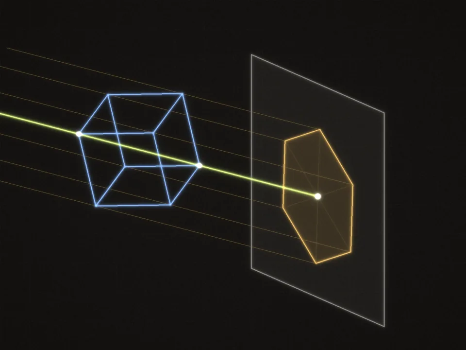A shadow squashes 3D onto a plane. A whole line of points, one ray of light, lands on each point of the wall: two dimensions survive and one is crushed.

Now count: 2 dimensions survive (the plane) and 1 is crushed (the line), and $2 + 1 = 3$, the number of input dimensions. That is always true.

In short: every input dimension is either kept (it counts toward the rank) or crushed (it counts toward the null space), never both and never neither.

#Solving with a singular matrix

In the last lesson, an invertible $\mathbf{A}$ meant exactly one solution to $\mathbf{A}\mathbf{x} = \mathbf{b}$. What happens when $\mathbf{A}$ cannot be inverted? The column space and the null space answer it. With the 3x3 matrix above:

• $\mathbf{b} = (2,\allowbreak 3,\allowbreak 5)$ lies in the plane $z = x + y$, since $2 + 3 = 5$. And $\mathbf{x} = (2,\allowbreak 3,\allowbreak 0)$ works: $2\mathbf{c}_1 + 3\mathbf{c}_2 = (2,\allowbreak 0,\allowbreak 2) + (0,\allowbreak 3,\allowbreak 3) = (2,\allowbreak 3,\allowbreak 5)$. So does $(2,\allowbreak 3,\allowbreak 0) + t\,(1,\allowbreak 1,\allowbreak -1)$ for every number $t$, because adding a null-space vector adds $\mathbf{0}$ to the output. For example $t = 1$ gives $(3,\allowbreak 4,\allowbreak -1)$, and $3\mathbf{c}_1 + 4\mathbf{c}_2 - \mathbf{c}_3 = (3,\allowbreak 0,\allowbreak 3) + (0,\allowbreak 4,\allowbreak 4) - (1,\allowbreak 1,\allowbreak 2) = (2,\allowbreak 3,\allowbreak 5)$. Infinitely many solutions: one particular solution plus the whole null space.
• $\mathbf{b} = (1,\allowbreak 1,\allowbreak 1)$ has $z = 1$ but $x + y = 2$. It is outside the column space, and no input lands there. No solution.

One more fact, stated without proof: the largest number of independent rows always equals the largest number of independent columns. That is surprising, since the rows and the columns live in different spaces, but it means rank is the same whether you look at rows or columns. An $m \times n$ matrix therefore has rank at most the smaller of $m$ and $n$: a $3 \times 1000$ matrix has only 3 rows, so its rank is at most 3, even though it has 1,000 columns. A matrix whose rank reaches that limit is called full rank.

For a square $n \times n$ matrix, all of the following say the same thing, and each one implies the others:

• $\det\mathbf{A} \ne 0$;
• $\mathbf{A}$ has an inverse;
• the columns are independent;
• the rank is $n$;
• the null space contains only $\mathbf{0}$;
• $\mathbf{A}\mathbf{x} = \mathbf{b}$ has exactly one solution for every $\mathbf{b}$.

Now read a rank off the columns of a wide matrix: walk through them and ask whether each one adds a new direction.

Next, go the other way: find a vector that a singular matrix crushes. Look for a relation between its columns, as we did for $\mathbf{c}_3 = \mathbf{c}_1 + \mathbf{c}_2$.

How a computer finds the rank

Spotting relations by eye works for small integer matrices. A computer needs a procedure. Walk through the columns and keep each one that adds a new direction. A column adds a new direction when it has a nonzero part perpendicular to all the columns kept so far, and projection from the dot product lesson finds that part: keep a set of perpendicular unit vectors that span the kept columns, remove the new column's shadow on each of them, and see whether anything is left.

On the 3x3 example:

1. $\mathbf{c}_1 = (1,\allowbreak 0,\allowbreak 1)$ is the first column, so keep it. Its unit vector is $\mathbf{q}_1 = (1,\allowbreak 0,\allowbreak 1)/\sqrt2$.
2. $\mathbf{c}_2 = (0,\allowbreak 1,\allowbreak 1)$. Its dot product with $\mathbf{q}_1$ is $\big((0)(1) + (1)(0) + (1)(1)\big)/\sqrt2 = \tfrac{1}{\sqrt2}$, so its shadow on $\mathbf{q}_1$ is $(\mathbf{c}_2\cdot\mathbf{q}_1)\,\mathbf{q}_1 = \tfrac{1}{\sqrt2}\cdot\tfrac{(1, 0, 1)}{\sqrt2} = \tfrac12(1,\allowbreak 0,\allowbreak 1) = (0.5,\allowbreak 0,\allowbreak 0.5)$. What is left is $(0,\allowbreak 1,\allowbreak 1) - (0.5,\allowbreak 0,\allowbreak 0.5) = (-0.5,\allowbreak 1,\allowbreak 0.5)$, which is not zero, so keep $\mathbf{c}_2$. Its unit vector $\mathbf{q}_2$ is $(-0.5,\allowbreak 1,\allowbreak 0.5)$ divided by its length, $\sqrt{1.5}$.
3. $\mathbf{c}_3 = (1,\allowbreak 1,\allowbreak 2)$. Its dot product with $\mathbf{q}_1$ is $\big((1)(1) + (1)(0) + (2)(1)\big)/\sqrt2 = \tfrac{3}{\sqrt2}$, so its shadow on $\mathbf{q}_1$ is $\tfrac{3}{\sqrt2}\cdot\tfrac{(1, 0, 1)}{\sqrt2} = \tfrac32(1,\allowbreak 0,\allowbreak 1) = (1.5,\allowbreak 0,\allowbreak 1.5)$, which leaves $(1,\allowbreak 1,\allowbreak 2) - (1.5,\allowbreak 0,\allowbreak 1.5) = (-0.5,\allowbreak 1,\allowbreak 0.5)$. That leftover is exactly the vector left over in step 2, so it points along $\mathbf{q}_2$: its shadow on $\mathbf{q}_2$ is all of it, and nothing is left. Skip $\mathbf{c}_3$.

Two columns kept: rank 2. np.linalg.matrix_rank uses a sturdier method based on singular values, which arrive in module 4. Now write the procedure yourself.

#Rank one and rank k

So far low rank has meant something lost. Now it becomes something gained: a matrix of low rank takes very few numbers to write down.

The simplest nonzero matrices have rank 1. Take a column vector $\mathbf{u}$ with $m$ entries and a column vector $\mathbf{v}$ with $n$ entries. Their outer product $\mathbf{u}\mathbf{v}^\top$ is the $m \times n$ matrix whose entry in row $i$ and column $j$ is $u_i v_j$. (The transpose $\mathbf{v}^\top$ is $\mathbf{v}$ laid on its side as a row, so $\mathbf{u}\mathbf{v}^\top$ is a column times a row, as in module 2.) For $\mathbf{u} = (1,\allowbreak 2)$ and $\mathbf{v} = (3,\allowbreak 1,\allowbreak 2)$, row 1 is $1 \times (3,\allowbreak 1,\allowbreak 2)$ and row 2 is $2 \times (3,\allowbreak 1,\allowbreak 2)$:

Every column is a multiple of $\mathbf{u}$ (3, 1 and 2 times it) and every row is a multiple of $\mathbf{v}^\top$ (1 and 2 times it). So the column space is the line through $\mathbf{u}$ and the rank is 1. Storing it takes the $m + n = 2 + 3 = 5$ numbers of $\mathbf{u}$ and $\mathbf{v}$ instead of all $mn = 6$ entries. For a $1000 \times 1000$ rank-one matrix that is 2,000 numbers instead of 1,000,000.

Sums of outer products. A sum of $k$ outer products,

where $\mathbf{U}$ is $m \times k$ with columns $\mathbf{u}_i$ and $\mathbf{V}$ is $n \times k$ with columns $\mathbf{v}_i$, has rank at most $k$. The reason: column $j$ of $\mathbf{M}$ is $v_{1j}\mathbf{u}_1 + \cdots + v_{kj}\mathbf{u}_k$ (with $v_{ij}$ meaning entry $j$ of $\mathbf{v}_i$), so every column is a combination of the same $k$ vectors. The equality on the right is the outer-product view of matrix multiplication from module 2: a product is the sum of (column $i$ of the left factor) times (row $i$ of the right factor). Storing $\mathbf{M}$ this way takes $k(m + n)$ numbers.

The converse is also true: every matrix of rank $k$ is a sum of $k$ outer products. Pick $k$ independent columns $\mathbf{c}_1,\allowbreak \ldots,\allowbreak \mathbf{c}_k$ of $\mathbf{M}$. They span the column space, because $k$ independent vectors inside a space of dimension $k$ reach all of it. So every column of $\mathbf{M}$ is a combination of them: column $j$ is $\sum_i r_{ij}\mathbf{c}_i$ for some numbers $r_{ij}$. Collect those numbers in a $k \times n$ matrix $\mathbf{R}$; then $\mathbf{M} = \mathbf{C}\mathbf{R}$ with $\mathbf{C} = [\mathbf{c}_1 \cdots \mathbf{c}_k]$, which is $k$ outer products, one for each column of $\mathbf{C}$ with the matching row of $\mathbf{R}$.

One more fact carries the rest of this lesson. If $\mathbf{B}$ is $m \times r$ and $\mathbf{A}$ is $r \times n$, then $\mathbf{B}\mathbf{A}$ has rank at most $r$, however large $m$ and $n$ are. The reason is the column view: each column of $\mathbf{B}\mathbf{A}$ is $\mathbf{B}$ times a column of $\mathbf{A}$, which is a combination of the $r$ columns of $\mathbf{B}$. All outputs live in a space of dimension at most $r$.

The run below builds a $6 \times 8$ matrix from two outer products, draws each layer as a heatmap (one colored cell per entry), and checks the ranks and the storage count.

Each rank-one layer is a pattern of stripes: one fixed row shape, repeated down the rows with different strengths. The sum has rank 2 and costs $2 \times (6 + 8) = 28$ numbers instead of 48.

A picture that is not built from a few layers can still be approximated by a few. The widget below does that for a $16 \times 16$ grid of brightness values, a smiley face, which is a matrix $\mathbf{A}$ with 256 entries between 0 (dark) and 1 (bright). $\mathbf{A}_k$ is a sum of $k$ rank-one layers. The widget picks the best possible layers, using the singular value decomposition from module 4; for now take that choice as given and watch what rank buys.

On screen: $\mathbf{A}$ on the left, $\mathbf{A}_k$ in the middle, and $\mathbf{A} - \mathbf{A}_k$ on the right, which is what is still missing (coral where $\mathbf{A}$ is brighter, blue where $\mathbf{A}_k$ overshoots, dark where they agree). Under them are the slider for $k$, the Build it up button and a sentence that says what changed. Below that, the last layer kept is drawn as a column times a row. The readouts give the relative error (the size of $\mathbf{A} - \mathbf{A}_k$ as a share of the size of $\mathbf{A}$), the numbers stored, $k(m + n)$, and the rank of A.

The face is exact at rank 8, not 16, because it is symmetric from left to right: column $j$ equals its mirror column, so at most 8 columns can be independent. Notice the price at that point. Eight layers of a $16 \times 16$ picture store $8 \times (16 + 16) = 256$ numbers, exactly as many as the picture itself. Factoring saves storage only while $k(m + n) < mn$: here $32k < 256$, so $k < 8$. Low rank pays off when $k$ is much smaller than both dimensions. For a small picture that is barely the case. For a $4096 \times 4096$ weight matrix in a language model the break-even rank is $4096 \times 4096 / 8192 = 2048$, and the ranks people use for LoRA are more like 8 or 16.

#LoRA: a low-rank change to the weights

Everything in this lesson comes together in one of the most widely used ways to fine-tune large language models. Fine-tuning means taking a pretrained model and adjusting its weights for a new task.

A pretrained layer has a weight matrix $\mathbf{W}_0$ of shape $d_{\text{out}} \times d_{\text{in}}$: in the column convention, it maps an input $\mathbf{x}$ with $d_{\text{in}}$ numbers to the output $\mathbf{W}_0\mathbf{x}$ with $d_{\text{out}}$ numbers. Full fine-tuning adjusts all $d_{\text{out}} d_{\text{in}}$ entries. LoRA (low-rank adaptation, Hu and colleagues, 2021) freezes $\mathbf{W}_0$ and learns only a change of the form

with a small rank $r$. ($\Delta$, the Greek capital delta, means "change in". $\mathbf{B}$ and $\mathbf{A}$ are the names the LoRA paper uses for the two factors; this $\mathbf{A}$ is not the matrix of the earlier sections.) The adapted layer computes $(\mathbf{W}_0 + \mathbf{B}\mathbf{A})\mathbf{x} = \mathbf{W}_0\mathbf{x} + \mathbf{B}\mathbf{A}\mathbf{x}$. Two facts from this lesson apply at once: $\mathbf{B}\mathbf{A}$ has rank at most $r$, and the two factors hold only $r(d_{\text{out}} + d_{\text{in}})$ numbers.

The diagram follows one tiny LoRA update through five steps: a $6 \times 6$ weight matrix and an update of rank 2. Each square is one entry, colored by its value (coral for positive, blue for negative, deeper for larger), with the number written on it. The shape and the count of numbers are written under each matrix ($\mathbf{A}$'s are to its right). Move through the steps with Next and Back, the step dots, or the arrow keys.

Three details follow from this lesson.

• Training starts from the pretrained model. $\mathbf{B}$ starts at zero (and $\mathbf{A}$ at small random values), so at the start $\Delta\mathbf{W} = \mathbf{B}\mathbf{A} = \mathbf{0}$ and the adapted layer gives exactly $\mathbf{W}_0\mathbf{x}$.
• The update is restricted, not small. It has rank at most $r$, so whatever the input, it adds a vector from one fixed $r$-dimensional subspace, the column space of $\mathbf{B}$. But the entries of $\mathbf{B}$ and $\mathbf{A}$ can be large, so along those few directions the change can be big.
• It costs nothing at run time. After training, $\mathbf{W}_0 + \mathbf{B}\mathbf{A}$ can be added up into one matrix (step 4 of the diagram), so the adapted model runs as fast as the original. Or $\mathbf{B}$ and $\mathbf{A}$ can be kept apart, so one base model can serve many small adapters.

Count the trainable numbers of an update yourself, this time for a rectangular matrix.

Now build a LoRA-style adapter in code, in the row convention numpy uses, and measure why the factored form is also cheaper to run.

To recap the lesson: rank counts the dimensions that survive; rank plus nullity is the number of columns; a rank-$k$ matrix is $k$ outer products and costs $k(m + n)$ numbers; and LoRA trains exactly such a matrix as the change to a frozen layer. Finish by explaining what that restriction does and does not mean.