A matrix is a function you can write down. Its columns record where the basis vectors land, and that is enough to know where every vector goes. Read row by row, the same numbers are a layer of neurons.
About 85 minutes
By the end you can
Test whether a map is linear by checking that it respects addition and scaling, the two operations from module 1.
Write the matrix of a transformation by finding where the basis vectors land.
Compute Ax two ways, as a combination of columns and as dot products with rows.
Derive the rotation matrix and recognize scales, stretches, shears, reflections, projections and singular matrices.
Read a layer of neurons as a matrix, one row of weights per neuron, and compute its outputs.
Implement matrix-vector multiplication both ways in Python.
Inside a language model, every token is carried as a vector, a list of a few thousand numbers like the ones in module 1, and each layer turns that vector into another vector. The machine that does most of that work is a matrix, a rectangular grid of numbers. This lesson is about what that machine does, and it starts with a small surprise.
Here is a rule that moves the points of the plane: send (x,y) to (2x−y,x+y). Try it on the two simplest points. The point (1,0) goes to (2⋅1−0,1+0)=(2,1), and the point (0,1) goes to (2⋅0−1,0+1)=(−1,1). Now, where does (3,2) go? You could substitute: (2⋅3−2,3+2)=(4,5). Or you could notice that (3,2) is 3 steps along (1,0) plus 2 steps along (0,1), and guess that it lands 3 steps along (2,1) plus 2 steps along (−1,1):
3(2,1)+2(−1,1)=(6,3)+(−2,2)=(4,5).
Same answer. That is not luck. For this kind of rule, the two answers for (1,0) and (0,1) decide where every other point goes. Write those two answers side by side as columns and you have the rule's matrix.
The lesson goes in four steps. First, what "this kind of rule" means: the rule has to be linear. Second, why two columns then decide everything. Third, a gallery of the common matrices, each read off from its columns. Fourth, a second way to read the same grid of numbers, row by row, which is exactly how a layer of neurons uses it.
The shortcut in the opening does not work for every rule. This section says which rules it works for, and what those rules look like.
In Arrows and lists you did two things with vectors: added them and scaled them. Write T (for transformation) for a function that turns vectors into vectors, and T(u) for the vector it produces from u. The function is linear when it respects both operations:
T(u+v)=T(u)+T(v),T(cu)=cT(u)
for all vectors u, v and every number c. In words: adding two inputs and then transforming gives the same result as transforming each and then adding; scaling before or after makes no difference either.
Check both rules on the opening rule, T(x,y)=(2x−y,x+y), with u=(1,0), v=(0,1) and c=3:
Addition. On the left, u+v=(1,1) and T(1,1)=(2−1,1+1)=(1,2). On the right, T(u)+T(v)=(2,1)+(−1,1)=(1,2). Equal.
Scaling. On the left, 3u=(3,0) and T(3,0)=(6−0,3+0)=(6,3). On the right, 3T(u)=3(2,1)=(6,3). Equal.
One check with particular numbers is not a proof, since the rules must hold for every input. The slow box does it for every input at once.
Go slower: Why the opening rule passes for every input
Write u=(u1,u2) and v=(v1,v2).
Step 1, add first.u+v=(u1+v1,u2+v2).
Step 2, apply the rule to that sum:
T(u+v)=(2(u1+v1)−(u2+v2),(u1+v1)+(u2+v2)).
Step 3, expand the brackets in the first entry: 2u1+2v1−u2−v2.
Step 4, sort the terms by where they came from, the u terms together and the v terms together: the first entry is (2u1−u2)+(2v1−v2) and the second is (u1+u2)+(v1+v2).
Step 5, read the groups.(2u1−u2,u1+u2) is T(u) and (2v1−v2,v1+v2) is T(v), so T(u+v)=T(u)+T(v).
Step 6, scale first.cu=(cu1,cu2).
Step 7, apply the rule to that: T(cu)=(2cu1−cu2,cu1+cu2).
Step 8, pull out c. Every term has a factor c, so take it out of each entry: (2cu1−cu2,cu1+cu2)=c(2u1−u2,u1+u2)=cT(u).
The same argument works whenever every output entry is a fixed weighted sum of the inputs, with no constant term and no products of inputs. That gives a quick test for linearity.
Put the two rules together and you get the version we will use all the time. For any numbers c1,c2 and vectors v1,v2, the addition rule splits the sum (first equals sign), and then the scaling rule pulls out each number (second equals sign):
A linear function carries linear combinations through unchanged. The recipe "this much of v1, that much of v2" survives the trip, with each ingredient replaced by its image. The opening used exactly this: (3,2)=3(1,0)+2(0,1), so T(3,2)=3T(1,0)+2T(0,1). That sentence is behind everything in this lesson.
What does linearity look like? Three things follow from the two rules:
The origin stays put. Take c=0 in the scaling rule: T(0)=T(0u)=0T(u)=0.
Straight lines stay straight, or collapse to a single point.
Parallel, evenly spaced grid lines stay parallel and evenly spaced. The square grid of the plane becomes a grid of identical parallelograms. It can be stretched, turned, flipped or flattened, but never bent.
Go slower: Why lines stay lines and spacing stays even
A line through the point p with direction d is the set of all points p+td, where t ranges over every number.
Step 1. Apply T and use the addition rule, then the scaling rule:
T(p+td)=T(p)+T(td)=T(p)+tT(d).
Step 2. Read the result. As t varies, T(p)+tT(d) traces the line through the point T(p) with direction T(d). If T(d)=0, every point of the line lands on the single point T(p).
Step 3, parallel lines. Two parallel lines share the direction d, so their images share the direction T(d): still parallel.
Step 4, even spacing. The points at t=0,1,2,3 are evenly spaced along the original line. Their images T(p),T(p)+T(d),T(p)+2T(d),… are evenly spaced too, one step of T(d) apart.
A grid is made of such lines, so a grid of squares becomes a grid of parallelograms.
Knowing what is not linear is just as useful. (Read the arrow ↦ as "goes to".) Each of these fails at least one rule, and one set of numbers is enough to show it:
Shifting, (x,y)↦(x+1,y). It sends (0,0) to (1,0), but a linear map must keep the origin fixed.
Products and powers of the inputs, such as (x,y)↦(xy,y). It sends (1,1) to (1,1) and (2,2) to (4,2). Doubling the input quadrupled the first output, where the scaling rule demands 2(1,1)=(2,2).
Bending: sin, tanh, the ReLU, applied to single numbers (vectors with one entry). The ReLU keeps positive numbers and turns negative ones into 0. It fails the addition rule: ReLU(−1+1)=ReLU(0)=0, but ReLU(−1)+ReLU(1)=0+1=1. The nonlinearities in a neural network are exactly the parts that break these rules, on purpose (Neurons and layers shows why they have to).
Left: a linear map. Grid lines stay straight, parallel and evenly spaced, and the origin stays put. Middle: a shift moves the origin, so it is not linear. Right: a map that bends the grid lines is not linear either, even though it keeps the origin in place.
Now test the two rules yourself on five maps. The quick test from the slow box (fixed weighted sums, no constants, no products) will do most of the work.
Quick checkWhich maps are linear?
Which of these maps of the plane are linear? Test each one against the two rules T(u+v)=T(u)+T(v) and T(cu)=cT(u). Select every linear one; more than one is.
The opening guessed that two answers decide where every point goes. Linearity turns that guess into a fact, and the fact hands us the matrix.
In the plane, the standard basis vectors from Arrows and lists, e1=(1,0) and e2=(0,1), are also written ^ and ^, read "i-hat" and "j-hat". Every vector is a combination of them: (x1,x2)=x1^+x2^. The coordinates are the coefficients. Now apply a linear T and let it carry the combination through, as the last section showed it must:
T(x)=T(x1^+x2^)=x1T(^)+x2T(^).
So once you know the two vectors T(^) and T(^), you know T everywhere. Write them down as the two columns of a grid of numbers. That grid is the matrix of T.
For the rule in the opening, T(^)=(2,1) and T(^)=(−1,1), so
A=[21−11],
and multiplying A by a vector is defined to mean that combination of its columns:
Ax=x1[21]+x2[−11]=[2x1−x2x1+x2].
With x=(3,2), the columns give 3(2,1)+2(−1,1)=(6−2,3+2)=(4,5), as before. (Inside sentences we write vectors in a row, like (3,2), to save space. In the math they are columns, which is why the columns of A stand upright in the grid.)
The widget below draws this matrix. It answers one question: if you know only where the two basis vectors land, can you find where any vector lands? On screen is the plane with its faint square grid. The blue arrow A^ ends at (2,1), the first column; the coral arrow A^ ends at (−1,1), the second column. The blue and coral lines are the whole grid after A has moved it. The dashed white arrow is the input v=(3,2) and the solid white arrow is its image Av.
Here is the general statement. A matrix with m rows and n columns is called m×n ("m by n"). Its entry in row i and column j is written Aij: row first, then column. Call its columns a1,…,an. For a vector x with n entries,
Ax=x1a1+x2a2+⋯+xnan.
There is one coefficient per column, so the input needs n entries. Each column has m entries, so the output has m. Writing Rn for the set of all vectors with n real entries, an m×n matrix is a function from Rn to Rm. Notice that the order flips: the number of columns (second in the shape) is the input size, and the number of rows (first) is the output size. A 3×2 matrix, for example, takes points of the plane to points in 3D. Its two columns are two arrows in 3D, and every output is a combination of them, so the whole plane lands on a flat sheet through the origin in 3D space (or on a line, if the two columns are parallel).
The logic also runs the other way: every matrix gives a linear function. Check the addition rule, one move per equals sign. As in module 1, ∑j means "add up over every j", here over the columns j=1,…,n, so Ax=∑jxjaj:
The first equals sign is the definition, since the entries of u+v are uj+vj. The second multiplies out each term. The third splits one sum into two. The last reads each sum as a matrix times a vector. Scaling is shorter: A(cu)=∑j(cuj)aj=c∑jujaj=cAu, pulling the common factor c out of every term. So "linear function" and "matrix" are two names for one thing, once you fix the basis. That is why this module is called Matrices are machines: a matrix is a function you can write down.
To recap: a linear map is decided by where the basis vectors land; those landing points are the columns of its matrix; and Ax takes x1 of the first column, x2 of the second, and so on.
The first exercise goes from a description in words to a matrix and back to a point, the way the opening did.
On paperWrite the matrix, then apply it
For each transformation, find where ^=(1,0) and ^=(0,1) land, write those two vectors as the columns of a 2×2 matrix, then apply the matrix to the given vector as a combination of its columns: (first entry) times column 1 plus (second entry) times column 2.
Rotate a quarter turn counterclockwise. Apply it to (2,1).
Reflect across the line y=x. Apply it to (3,−1).
Stretch horizontally by 3 and turn the plane upside down (every y becomes −y). Apply it to (1,2).
The shear that keeps ^ where it is and slides ^ to (2,1). Apply it to (1,1).
To check, enter the four images in order, one per row, as x then y.
Work it on real paper: writing each step is the point. Then check your final answer here and compare your working with the walk-through.
The four images in order, one per row: x, then y
One entry per box, row by row (Tab moves along a row). 0.25, -2, 3/4 and sqrt(2) all work. Enter moves to the next empty box and checks once all are filled.
The next one gives you clues about two vectors that are not both basis vectors, so you have to use linearity to find the missing column.
Work it outA matrix from two clues
A linear map sends (1,0) to (2,1) and sends (1,1) to (1,3). Find its matrix. You are not told directly where (0,1) goes. Enter the 2×2 matrix row by row.
A
One entry per box, row by row (Tab moves along a row). 0.25, -2, 3/4 and sqrt(2) all work. Enter moves to the next empty box and checks once all are filled.
Most matrices you will meet are built from a handful of basic moves: scaling, stretching, shearing, rotating, reflecting and flattening. Each one is easiest to recognize by where it sends ^ and ^, so it is worth seeing each one move the grid once.
The widget below starts at the identity, the matrix that moves nothing, and has one button per move. On screen are the faint original grid, the moved grid, the blue and coral arrows (the two columns, which you can also read in the matrix cells: blue cells are column 1, coral cells column 2), and the unit square, the square with corners (0,0), (1,0), (1,1) and (0,1). Where it lands is shaded, and the area readout gives the shaded area. The sentence under the t slider names the move.
Every entry in this table comes from the same question, where do ^ and ^ go. The two middle columns of the table are the two columns of the matrix. The letter k stands for any amount you choose.
Transformation
^ lands at
^ lands at
Matrix
Scale everything by k
(k,0)
(0,k)
[k00k]
Stretch horizontally by k
(k,0)
(0,1)
[k001]
Shear sideways by k
(1,0)
(k,1)
[10k1]
Rotate by θ
(cosθ,sinθ)
(−sinθ,cosθ)
[cosθsinθ−sinθcosθ]
Reflect across the x-axis
(1,0)
(0,−1)
[100−1]
Reflect across y=x
(0,1)
(1,0)
[0110]
Project onto the x-axis
(1,0)
(0,0)
[1000]
Squash onto a line (singular)
(1,2)
(2,4)
[1224]
Three of these deserve a closer look.
Rotation. The unit circle is the circle of radius 1 around the origin, and the point on it at angle α (measured counterclockwise from the positive x-axis) is (cosα,sinα): that is the definition of cosine and sine. Rotating counterclockwise by θ carries ^, which sits on the unit circle at angle 0, to the point at angle θ, which is (cosθ,sinθ). The vector ^ starts a quarter turn ahead, at angle 90∘, so it lands at angle θ+90∘, which is the point (−sinθ,cosθ). Those are the two columns.
Go slower: Where ^ lands under a rotation
The point on the unit circle at angle α is (cosα,sinα). For ^ after the rotation, α=θ+90∘. Use the angle-addition formulas, then cos90∘=0 and sin90∘=1:
cos(θ+90∘)=cosθcos90∘−sinθsin90∘=cosθ⋅0−sinθ⋅1=−sinθ,sin(θ+90∘)=sinθcos90∘+cosθsin90∘=sinθ⋅0+cosθ⋅1=cosθ.
So ^ lands at (−sinθ,cosθ). A shortcut that gives the same answer: turning any vector (a,b) a quarter turn counterclockwise gives (−b,a), and the image of ^ is the image of ^, (cosθ,sinθ), turned a further quarter turn.
Two angles as examples. For θ=90∘, cosθ=0 and sinθ=1, so the columns are (0,1) and (−1,0): the matrix [01−10] you saw in the widget. For θ=30∘, cosθ=3/2≈0.866 and sinθ=1/2, so the matrix is [3/21/2−1/23/2]≈[0.8660.5−0.50.866]. It sends (2,0) to 2 times the first column, 2(3/2,1/2)=(3,1)≈(1.732,1). Its length is (3)2+12=3+1=2, the same as before, as a rotation should leave it.
Projection. The projection onto the x-axis keeps the x-part of every vector and throws away the y-part, so ^ lands on 0. Projections onto other lines are matrices too. In The dot product you found that the projection of a onto the line through b is b⋅ba⋅bb. Take b=(1,1). Then b⋅b=1+1=2 and a⋅b=a1+a2, so the projection is 2a1+a2(1,1). For ^=(1,0) that is 21+0(1,1)=(21,21), and for ^=(0,1) it is 20+1(1,1)=(21,21) as well. So the matrix is [1/21/21/21/2]. Check it on a=(4,2) from that lesson's exercise: 4(21,21)+2(21,21)=(2,2)+(1,1)=(3,3), the same projection you computed there. Applying the matrix a second time changes nothing: 3(21,21)+3(21,21)=(3,3). The point is already on the line, so its shadow is itself.
Singular matrices. In [1224] the second column is twice the first. (The widget's Singular preset uses a different pair with the same property, columns (1,0.5) and (2,1).) Every output is x1(1,2)+x2(2,4). Replace (2,4) by 2(1,2) and collect the two multiples of (1,2):
x1(1,2)+x2⋅2(1,2)=(x1+2x2)(1,2).
So every output is a multiple of (1,2), and the whole plane is squashed onto the line through (1,2). Different inputs collide. For (1,1) the multiple is 1+2⋅1=3, and for (3,0) it is 3+2⋅0=3, so both land on 3(1,2)=(3,6). For (2,−1) it is 2+2⋅(−1)=0, so it lands on the origin. Once two inputs share an output, nothing can tell you which one you started from, so no matrix can undo this one. Module 3 measures this collapse with the determinant and counts the surviving dimensions with rank.
To recap the gallery: every matrix in it came from the one question, where do ^ and ^ land. Rotations and shears keep areas, reflections flip the plane over, and a matrix whose columns lie on one line flattens the plane and cannot be undone.
Now read a matrix straight off a picture, the way you read the presets.
Quick checkRead the matrix off the picture
In the transformation widget you see this picture: the blue arrow, the image of ^, ends at (1,1). The coral arrow, the image of ^, ends at (−1,1). The unit square has become a larger square, turned 45∘ counterclockwise. Which matrix is on the screen?
The column view says what a matrix does to the plane. There is a second way to read the same arithmetic, and it is the one a neural network uses, so it is worth deriving carefully. Write Ax out entry by entry for a 2×2 matrix. The first equals sign is the column view; the second multiplies each column by its number and adds the two columns entry by entry:
Now look at the top entry, A11x1+A12x2. It uses only the first row of A, (A11,A12), and it multiplies matching entries and adds: it is (A11,A12)⋅(x1,x2), row 1 dotted with x. The bottom entry is row 2 dotted with x. In general, writing (Ax)i for entry i of the vector Ax, and with ∑j=1n meaning "add up for j=1,2,…,n",
(Ax)i=j=1∑nAijxj=(row i of A)⋅x.
Both views compute the same terms Aijxj; they only group them differently. The row view fixes the output entry i and adds along the row. The column view collects every term that shares the same xj, which gives xj times column j.
Check it on the opening example. The rows of A=[21−11] are (2,−1) and (1,1). With x=(3,2), the first entry is (2)(3)+(−1)(2)=6−2=4 and the second is (1)(3)+(1)(2)=3+2=5. The same (4,5) we built from the columns.
Each view earns its keep:
The row view is how you compute by hand, and how you think about each output separately. Every row is a pattern, and output i measures how much x lines up with pattern i: large and positive when they agree, zero when they are perpendicular, negative when they disagree. That is the dot product's meaning, from The dot product.
The column view is how you see geometry. Every output is a combination of the columns, so the outputs can only ever reach the span of the columns (module 1). In module 3 that set gets a name, the column space.
A layer of neurons is a matrix
"Every row is a pattern" is not a figure of speech. It is exactly what a layer of a neural network is, and this is the first place in the course where a matrix meets one.
A neuron takes a list of numbers x, multiplies each by its own weight, adds the products, and adds one more number, its bias: it computes w⋅x+b, where w is its weight vector and b its bias. A layer is several neurons reading the same input, each with its own weights and bias. Stack the weight vectors as the rows of a matrix W and the biases into a vector b, and the row view says that Wx+b computes every neuron at once. (In a network a nonlinearity such as the ReLU then acts on each output. This lesson leaves it aside; Layers and parameter counts adds it.)
The diagram below answers the question: how does a grid of numbers become a layer of neurons? It has two parts, side by side on a wide screen and one above the other on a phone. The network drawing shows three inputs x1,x2,x3 (blue circles holding 2, 1 and −1) joined by lines to two neurons (white circles), one weight per line, with the biases b1=1 and b2=2 written beside the neurons. The equation shows the same layer as Wx+b=z, with each shape (rows × columns) written under its bracket. Move through it with Next and Back, or the numbered dots.
In matrix language, a layer of m neurons that each read n inputs is an m×n weight matrix: one row per neuron, one column per input. Now compute one yourself, with three neurons this time and two inputs.
Work it outThree neurons, three dot products
A layer of three neurons has weight rows (1,2), (0,−1) and (3,1), stacked into W=1032−11. There is no bias. Compute Wx for x=(2,−1) with the row view: one dot product per neuron. Enter the three outputs as a column, neuron 1 at the top.
Wx
One entry per box, top to bottom. 0.25, -2, 3/4 and sqrt(2) all work. Enter moves to the next empty box and checks once all are filled.
Writing each view as a loop forces you to say which index moves, and that is exactly the difference between them: the row view moves along a row for each output entry, and the column view adds one whole column per input entry.
Here are both views in numpy, and the 30∘ rotation from the gallery. Note that numpy counts from 0: A[0] is the first row and A[:, 0] is the first column. The first three lines should all print [4. 5.], and the rotation should send (2,0) to about (1.732,1), of length 2.
⌘+Enter runs · edit freelyPython sleeps until you run code
Now write both views yourself, without numpy's @, and build a rotation matrix from where the basis vectors go.
Code itMatrix times vector, both ways
Write matrix-vector multiplication twice, without @ or np.dot, so that both views from this lesson become code.
matvec_rows(A, x): entry i is row i of A dotted with x.
matvec_cols(A, x): x[0] times column 0, plus x[1] times column 1, and so on.
Both raise ValueError when x does not have one entry per column of A, and both work for non-square matrices.
rotation(theta) returns the 2×2 matrix that rotates counterclockwise by theta radians, built from where ^ and ^ land.
In numpy, A[i] is row i, A[:, j] is column j, and indices start at 0 (the math starts at 1).
⌘+Enter runsPython sleeps until you run code
Write your code where the starter says raise NotImplementedError, then press Run tests. Each check says what it expects.
A few quick reps by hand, with new numbers each time, make the row view automatic.
Practice setMatrix-vector reps
3 correct in a row completes the set. A miss starts the count again.
Compute Ax for A=[−2−111−3−3] and x=21−2.
Ax
One entry per box, top to bottom. 0.25, -2, 3/4 and sqrt(2) all work. Enter moves to the next empty box and checks once all are filled.
To recap the lesson: a matrix is a linear map; its columns are where the basis vectors land, so Ax is a combination of the columns; and read row by row, the same product is a stack of dot products, which is a layer of neurons. To finish, put the whole idea into your own words.
In your own wordsMore than a table of numbers
A colleague says a matrix is just a table of numbers. Explain what the columns of a 2×2 matrix mean geometrically, why those two columns are enough to know where every vector goes, and what the row view adds.


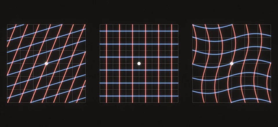 Left: a linear map. Grid lines stay straight, parallel and evenly spaced, and the origin stays put. Middle: a shift moves the origin, so it is not linear. Right: a map that bends the grid lines is not linear either, even though it keeps the origin in place.