Preferences, rewards and adapters

In the previous lesson you fine-tuned a small Shakespeare model on chat replies. It learned how a reply starts, and it lost some of its Shakespeare along the way. The method you used, supervised fine-tuning, has two limits. It can only imitate: someone has to write every ideal answer, the model never sees what a worse answer looks like, and it can only become as good as the people who wrote the examples. And the way you ran it trains every weight, which for a large model takes several times the memory of the weights themselves.

The methods in this lesson get around those limits. First, learning from comparisons, because picking the better of two answers is quicker than writing an ideal one: a reward model, RLHF and DPO. Second, learning from answers a program can check, which is central to training reasoning models. Third, two jobs that reuse the same objectives: safety tuning and distillation. Fourth, LoRA, which fine-tunes by training a small, low-rank change to each weight matrix. The lesson ends with what a post-training company does all day, including how it measures whether a change helped.

The pipeline widget from the big picture opens here at stage 6, Preferences, the first stage on the rail whose loss is not the cross-entropy of a given text. As before, the panel under the rail says what goes in and comes out, shows the loss in a pink box, and gives a small example.

The sections follow the rail: preferences, then checkable rewards, then two more uses of the same objectives, then LoRA, which works with any of them.

#Learning from preferences

Comparing two answers is quicker than writing an ideal one, and it teaches something imitation cannot: which of two plausible answers is better. Show a person (or a judging model) two answers to the same prompt $x$ and ask which is better. Call the preferred one $y_w$ and the other $y_l$ (for "win" and "lose").

The data diagram from the previous lesson opens below at step 3, one such comparison. The track at the top lights the current stage, lime marks the chosen answer, and coral the rejected one.

A reward model turns comparisons into a score. It is a network, often the SFT model with its output layer replaced by a single number, that maps a prompt and a response to a reward $r_\phi(x,\allowbreak y)$, where $\phi$ are its parameters. The Bradley-Terry model says the preferred response wins with probability $\sigma(r_\phi(x,\allowbreak y_w) - r_\phi(x,\allowbreak y_l))$, where $\sigma$ is the sigmoid. Training maximizes the likelihood of the observed choices:

Step 3 of the diagram is one such pair. The rewards are $1.2$ for the chosen answer and $0.4$ for the rejected one. Their difference is $0.8$, so the reward model gives the observed choice the probability $\sigma(0.8) = 1/(1 + e^{-0.8}) \approx 1/1.449 \approx 0.690$, and the loss is $-\ln 0.690 \approx 0.371$. Training pushes the difference up, which pushes the loss toward 0. Only the difference matters: adding the same constant to every reward changes nothing, so rewards have no fixed zero point.

RLHF (reinforcement learning from human feedback) then trains the language model, now called the policy $\pi_\theta$, to produce high-reward responses without drifting far from a frozen reference model $\pi_{\text{ref}}$, usually the SFT model:

Here $\mathbb{E}_{y \sim \pi_\theta}$ is the average over responses sampled from the policy, $\operatorname{KL}(\pi \,\|\, \pi_{\text{ref}}) = \sum_y \pi(y)\ln\frac{\pi(y)}{\pi_{\text{ref}}(y)}$ is the Kullback-Leibler divergence, which is zero when the two distributions agree and positive otherwise, and $\beta > 0$ sets how much drift costs. The penalty matters. A reward model is only an imperfect stand-in for human judgment, and a policy pushed hard against it finds responses that score well for the wrong reasons, an effect called reward hacking. Sampling is not differentiable, so the gradient is estimated from sampled responses with the policy gradient, derived in the section on verifiable rewards below. The classic algorithm for this step is PPO (Schulman and colleagues, 2017), used in the SFT, reward model, PPO pipeline that Ouyang and colleagues (2022) described for instruction-following models. It is demanding: training needs the policy, the reference, the reward model and a value model (an estimate of expected reward) at once.

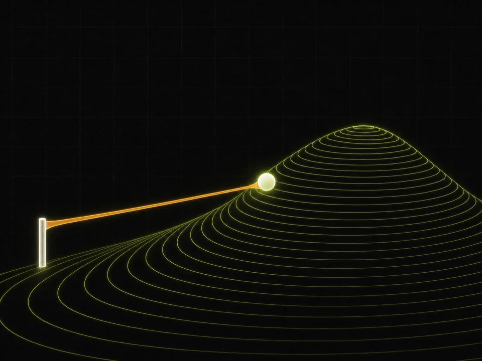The RLHF objective as a tether. The reward pulls the policy up the hill, and the KL penalty pulls it back toward the reference model, harder the further it drifts. The best policy sits in between, and closer to the post when β is larger.

DPO (direct preference optimization, Rafailov and colleagues, 2023) targets the same optimum without a reward model and without sampling during training. Write $\ln\pi(y \mid x)$ for the log-probability of a whole response, the sum of its tokens' log-probabilities (the chain rule from the big picture). The loss for one pair is

Each log-ratio measures how much the model has raised a response's probability compared with where it started. The loss is small when the preferred response has been raised more than the rejected one. It is a classification loss on fixed pairs of text, which is why DPO is so much simpler to run than RLHF.

The gradient explains how DPO behaves. Write $m$ for the quantity inside the sigmoid, so the loss for one pair is $-\ln\sigma(m)$. Its derivative with respect to $m$ is $-\sigma(-m)$, derived line by line below. Inside $m$, only the policy's log-probabilities depend on $\theta$, since the reference model is frozen, so the chain rule gives

A gradient-descent step moves against this, so it raises $\ln\pi_\theta(y_w \mid x)$ and lowers $\ln\pi_\theta(y_l \mid x)$, and each of those is a sum over the response's tokens, trained through the same per-token gradients as cross-entropy. The pair's weight is $\sigma(-m)$: above one half when the model currently favors the rejected response relative to the reference ($m < 0$), approaching 1 the more wrongly it ranks the pair, and close to 0 once it strongly favors the preferred one.

To recap: a reward model learns scores whose difference predicts which answer people prefer, and RLHF optimizes the policy against it while the KL penalty holds it near the reference. DPO applies the same sigmoid-of-a-difference loss directly to the policy's log-ratios. The next exercise computes one DPO loss.

#Rewards you can check

Preferences need a judge, a person or a model. Some tasks need only a checker: a math problem with a known answer, code with unit tests, a puzzle with a verifiable solution. Reinforcement learning with verifiable rewards uses the checker as the reward, as in step 4 of the data diagram above. For each prompt, sample $G$ attempts from the current model, score each with $R_i = 1$ if it passes and $0$ if not, and update the model to make passing attempts more likely. Reasoning models are trained this way at large scale: the model writes out intermediate steps before its answer, only the answer is checked, and the steps that led to correct answers become more likely.

The update comes from the policy gradient. In words: the gradient of the average reward equals the average, over attempts sampled from the model, of each attempt's reward times the gradient of that attempt's log-probability. (The box below derives it.)

In practice the reward is replaced by an advantage: how much better the attempt did than a baseline. With the group's average as the baseline, $A_i = R_i - \bar{R}$ where $\bar{R} = \frac{1}{G}\sum_j R_j$, and the step is $\theta \leftarrow \theta + \eta\,\frac{1}{G}\sum_i A_i\,\nabla_\theta\ln\pi_\theta(y_i)$.

Step 4 of the diagram is an example. Four attempts at "What is 7 × 8?" get rewards $(1,\allowbreak 0,\allowbreak 0,\allowbreak 1)$. Their mean is $\bar{R} = (1 + 0 + 0 + 1)/4 = 0.5$, and subtracting it from each reward gives the advantages $(+0.5,\allowbreak -0.5,\allowbreak -0.5,\allowbreak +0.5)$: the two successes are made more likely and the two failures less likely. If all four pass, or all four fail, every advantage is 0 and the prompt teaches nothing, so useful training prompts are the ones the model solves only some of the time. And because $\ln\pi_\theta(y) = \sum_t \ln\pi_\theta(y_t \mid x,\allowbreak y_{<t})$, each term is the cross-entropy gradient on the model's own attempt, scaled by its advantage: imitate your own successes, move away from your own failures.

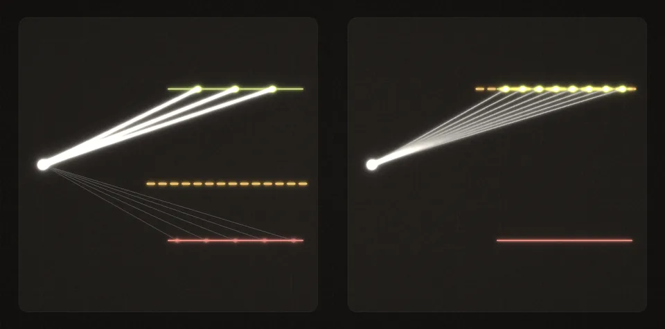Group-relative advantages. Left: attempts that pass sit above the group's average and become more likely, and attempts that fail sit below it and become less likely. Right: when every attempt passes, each one equals the average, so nothing changes.

Production algorithms add more. PPO-style methods clip each update so that a single batch cannot move the policy far. GRPO (Shao and colleagues, 2024) uses the group-relative advantage above, divided by the group's standard deviation, and many setups keep a KL penalty toward a reference model.

To recap: with a checker, the model learns from its own attempts, pushing each attempt's log-probability up or down in proportion to how much better it did than the group's average. The next question asks you to recognize this stage from a description.

#Two more tools: safety tuning and distillation

Two more jobs reuse the same objectives: teaching a model where the boundaries are, and moving what a large model knows into a small one.

Safety tuning uses all three kinds of training signal you have now seen: demonstrations of declining harmful requests and helping with harmless ones (a few are in chat-sft.txt, the file you fine-tuned on in the previous lesson), preference pairs that penalize both harmful compliance and needless refusal, and rule-based or model-graded rewards. The hard part is the boundary, which is why evaluations measure over-refusal as well as harm.

Distillation trains a smaller student to imitate a larger teacher: either SFT on the teacher's generated responses, or matching the teacher's whole next-token distribution $\mathbf{q}$ at every position with $L = -\sum_v q_v\ln p_v$, an approach popularized by Hinton, Vinyals and Dean (2015). The gradient with respect to the student's logits $\mathbf{z}$ is $\mathbf{p} - \mathbf{q}$: the $\mathbf{p} - \mathbf{y}$ of module 6 with the one-hot target replaced by the teacher's probabilities. The derivative of a log-softmax is $\partial \ln p_v/\partial z_j = \delta_{vj} - p_j$, where $\delta_{vj}$ is 1 when $v = j$ and 0 otherwise. So

using $\sum_v q_v = 1$ in the last step. A soft target carries more information per example than a single correct token, since it also says which wrong answers were nearly right.

To recap: safety tuning aims demonstrations, preferences and rewards at one boundary, and is measured on both sides of it. Distillation is cross-entropy with the teacher's distribution in place of the one-hot target, so its gradient is $\mathbf{p} - \mathbf{q}$.

#LoRA: fine-tuning a few directions

Every method so far can train every weight of the model, which is called full fine-tuning. Adam keeps two running averages for every weight it trains (you implemented them in module 6), so the memory for gradients and optimizer state is several times the memory of the weights themselves. A common mixed-precision setup keeps 16-bit weights and gradients plus 32-bit copies of the weights and both averages: about 16 bytes per trained parameter, against 2 for the weights alone. For large models that is the binding constraint. LoRA (low-rank adaptation, Hu and colleagues, 2021), which you met in module 3, freezes each pretrained matrix $\mathbf{W}_0$ and trains only a low-rank change. In the column convention of that lesson, $\Delta\mathbf{W} = \mathbf{B}\mathbf{A}$ with $\mathbf{B}$ of shape $d_{\text{out}} \times r$ starting at zero and $\mathbf{A}$ of shape $r \times d_{\text{in}}$ starting random, where the rank $r$ is small, often 8 to 64.

The diagram from that lesson draws a small case: a $6 \times 6$ pretrained matrix and a rank-2 update. Each square is one entry, coral for positive and blue for negative, and under each matrix are its shape and how many numbers it holds or trains.

In code, with rows as tokens, every matrix is transposed and the layer is

where $\mathbf{X}$ is $(B,\allowbreak d_{\text{in}})$ for a batch of $B$ tokens, $\mathbf{W}_0$ is now $d_{\text{in}} \times d_{\text{out}}$, $\mathbf{D} = \mathbf{A}^\top$ (for "down", shape $d_{\text{in}} \times r$) squeezes each input to $r$ numbers, $\mathbf{U} = \mathbf{B}^\top$ (for "up", shape $r \times d_{\text{out}}$) starts at zero, and $s$ is a fixed scale ($\alpha/r$ in the paper's notation).

The gradients follow from the linear-layer rule of backpropagation: for $\mathbf{Y} = \mathbf{X}\mathbf{W}$ with upstream gradient $\partial L/\partial\mathbf{Y}$, the weight gradient is $\mathbf{X}^\top(\partial L/\partial\mathbf{Y})$ and the input gradient is $(\partial L/\partial\mathbf{Y})\,\mathbf{W}^\top$. Let $\mathbf{G} = \partial L/\partial\mathbf{P}$ and $\mathbf{H} = \mathbf{X}\mathbf{D}$. The adapter path is a linear layer $\mathbf{H} = \mathbf{X}\mathbf{D}$ followed by a linear layer $s\,\mathbf{H}\mathbf{U}$, so the rule applied twice, from the output back, gives

At the start $\mathbf{U} = \mathbf{0}$, so $\partial L/\partial\mathbf{D} = \mathbf{0}$: only $\mathbf{U}$ moves on the first step, and $\mathbf{D}$ starts moving once $\mathbf{U}$ is nonzero. If both started at zero, both gradients would be zero forever. That is why one factor starts random.

The savings. A rank-$r$ adapter on a $d_{\text{in}} \times d_{\text{out}}$ matrix trains $r(d_{\text{in}} + d_{\text{out}})$ numbers. Suppose a model has 32 layers, each with four $4096 \times 4096$ attention matrices, and gets rank-16 adapters on all of them. That is $32 \times 4 \times 16 \times 8192 = 16{,}777{,}216$ trainable numbers, against $32 \times 4 \times 4096^2 = 2{,}147{,}483{,}648$ in those matrices: $0.78\%$. After training, the change can be merged into the weights, $\mathbf{W}_0 + s\,\mathbf{D}\mathbf{U}$, so the adapted model runs exactly as fast as the original. Or the adapters can be kept separate, so one base model serves many customers, each with a small adapter.

What rank $r$ can and cannot do. Whatever the input, the adapter's contribution to an output row, $s\,(\mathbf{x}\mathbf{D})\,\mathbf{U}$, is a combination of the $r$ rows of $\mathbf{U}$, so it lies in a space of at most $r$ dimensions. If the change a task needs has rank at most $r$, the adapter can learn it exactly. If not, the best it can do, when the inputs are spread evenly in every direction, is the best rank-$r$ approximation of the needed change, which module 4 showed is the truncated SVD. The code exercise below lets you watch gradient descent find exactly that. Whether real adaptations are low rank is an empirical question. For many tasks rank 8 to 64 comes close to full fine-tuning; published comparisons have also found that LoRA tends to learn less of a genuinely new domain than full fine-tuning, and to forget less of the old one.

To recap: LoRA freezes $\mathbf{W}_0$ and trains a rank-$r$ change $\mathbf{B}\mathbf{A}$, which costs $r(d_{\text{in}} + d_{\text{out}})$ numbers instead of $d_{\text{in}}d_{\text{out}}$, can be merged afterwards, and can represent any change of rank at most $r$. First count the savings for a real configuration.

Then train an adapter and see the rank limit for yourself.

#What a post-training company does

A company that does only post-training, like the one in the big picture, works on five things, and only one of them is running training code.

• Data. Collecting demonstrations from domain experts, generating candidates with strong models and filtering them, collecting preference pairs, and writing the guidelines that say what a good answer is. Most of the quality comes from here.
• Evaluation. Held-out test sets for the customer's tasks, automatic checkers where answers can be verified, rubrics and model-based judges where they cannot (with checks that the judge agrees with people), and regression tests on general abilities to catch forgetting. The three losses of your fine-tuning run in the previous lesson (the trained replies, the held-out replies and Shakespeare) were a tiny version of this.
• Training runs. SFT and LoRA or full fine-tuning on an open-weight base model, with sweeps over the learning rate, the number of steps and the data mixture. Then preference optimization or reinforcement learning where it pays off.
• Reward and verification infrastructure. Reward models, unit-test sandboxes for code, answer checkers, and the rules for safety behavior.
• Serving. Merging or hot-swapping adapters, quantizing, and meeting latency and cost targets, because a model that is too slow or expensive is not a product.

The last exercise asks you to say all of this to someone who has to decide whether to pay for it.