
Lesson 3 of 5
Pretraining and fine-tuning
Pretraining is the next-character loss you already wrote, run on trillions of tokens. Supervised fine-tuning keeps that loss and changes the data. This lesson writes out both, estimates what pretraining costs, and fine-tunes a model of your own.
Derive the compute estimate and use it to size a training run.
Say what scaling laws predict and what they do not, and what a base model can and cannot do.
Write the supervised fine-tuning loss with loss masking, and read the mask at the target positions.
Implement a masked fine-tuning loss, fine-tune a pretrained character model on chat data, and measure what it forgets.

In module 8 you trained a character LSTM on Shakespeare. At every position it predicted the next character, the loss was the cross-entropy of the character that actually came next, and Adam nudged tens of thousands of parameters to lower it. That was pretraining, and not as an analogy. Frontier language models are pretrained with the same objective. Three things change: tokens are pieces of words instead of characters, the network is a transformer instead of an LSTM, and the text runs to trillions of tokens instead of a hundred thousand characters.
Post-training comes afterwards: it takes a pretrained model and changes its behavior with far less data and compute, and it is what a post-training company sells. Its first stage, supervised fine-tuning, keeps pretraining's loss and changes only the data. So the loss you already know carries a model all the way from random weights to one that answers in a chat format. This lesson writes that loss out for both stages, estimates what pretraining costs before anyone starts a run, and has you fine-tune your own Shakespeare model into a (very small) assistant, watching what it gains and what it loses.
The widget from the big picture lays out the whole lifecycle of a language model as eight stages on a rail. Pretraining is selected. The panel under the rail says what goes in and comes out, the loss in a pink box, the rough scale, and a small example.
This lesson follows the rail from stage 3 to stage 5: pretraining and what it costs, the base model it produces, and supervised fine-tuning, which you then run on a model of your own. The next lesson, Preferences, rewards and adapters, takes stages 6 and 7 and a cheaper way to fine-tune.
Pretraining: the loss you already wrote
Take a training sequence of tokens . At each position the model reads and outputs a probability for every token in the vocabulary. The loss is the average surprise at the true next token:
where stands for all the parameters and is the softmax of the model's logits. This is exactly the loss of module 7, whose gradient with respect to the logits at each position is the of module 6, divided by for the average. The transformer of Inside a transformer computes all predictions of a sequence at once, using the causal mask.
Tokens. The are subword tokens, such as the byte-pair pieces of Inside a transformer, from a vocabulary of tens of thousands to a few hundred thousand. Ordinary English prose comes to roughly four characters per token, so a trillion tokens is about four trillion characters of text.
Data. Web pages, books, code, papers and more, filtered for quality, deduplicated, and mixed in chosen proportions. Data work is a large share of the effort.
The base model. Pretraining produces a model of documents. Given a question it may answer, or it may continue with three more questions, as the documents it learned from often do. It has absorbed facts, grammar, code and styles of writing because predicting text well requires them. It has no particular inclination to be helpful, honest or brief, beyond what its training documents happen to show. You can often steer it by writing the start of the document you want, for example a few question and answer pairs followed by your question.
To recap: pretraining is next-token cross-entropy over an enormous, filtered corpus of subword tokens, and it produces a base model that continues documents. The next question is what that costs.
How much compute: C is about 6ND
Before a pretraining run starts, one short formula estimates its cost. Write for the number of parameters, for the number of training tokens and for the total floating-point operations (FLOPs), counting one multiplication or one addition as one FLOP. The standard estimate is
The 6 comes from matrix multiplication, which is almost all of the work. Look at one linear layer with a weight matrix of shape , so parameters, applied to a batch of tokens, shape .
- Forward: has entries, and each is a sum of products, so it takes multiply-adds, the cost rule from module 2. Divide by the parameters and the tokens: multiply-add per parameter per token, or 2 FLOPs.
- Backward: backpropagation needs two products of the same size. is times , and is times . Each takes multiply-adds: 4 FLOPs per parameter per token together.
Forward plus backward is FLOPs per parameter per token. Almost every parameter of a transformer sits in such a matrix and is used once per token, so the whole run costs about .
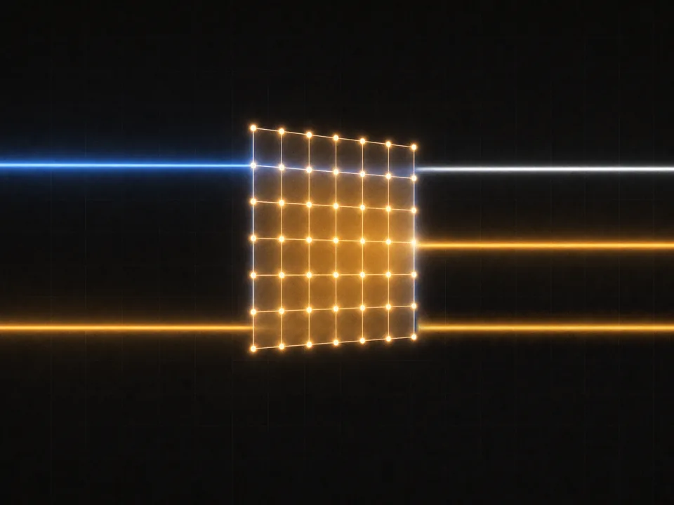 One product going forward and two coming back, all the same size. The inputs' gradient passes back through the weights, and the weights' gradient lands on the weights themselves: 2 + 4 = 6 FLOPs per parameter per token.
A worked example. A model with parameters trained on tokens needs
Suppose a GPU sustains FLOPs per second (the same assumption as in the big picture). Divide: GPU-seconds. Divide by 3,600 seconds per hour: about 83 hours on one GPU, or hours on eight. For scale, the character model you are about to pretrain has parameters and sees characters, so it costs FLOPs. The hypothetical 70-billion-parameter run in the big picture, FLOPs, is roughly times more.
Scaling laws, stated honestly. Kaplan and colleagues (2020) found that the pretraining loss falls smoothly, as a power law, as parameters, data and compute grow, over many orders of magnitude, as long as the other two are not the bottleneck. Hoffmann and colleagues (2022) asked how to split a fixed compute budget and found that parameters and tokens should grow together, with roughly 20 tokens per parameter as the compute-optimal ratio in their experiments. The worked example above is that split. Put into : . With , that gives , so , and . Many released models are trained on far more tokens per parameter than that, because a smaller model is cheaper to serve. The limits of these laws matter as much as the laws: they are curves fitted over the range that was measured, they predict the average loss rather than whether any particular skill appears, and they assume data of similar quality throughout.
To recap: training costs about 6 FLOPs per parameter per token, 2 forward and 4 backward, because every weight matrix takes part in one product going forward and two coming back. Multiply by and and divide by a GPU's speed to size a run.
The first exercise derives the 6 yourself, one product at a time.
A linear layer has a weight matrix of shape and processes a batch of tokens, shape . Count one multiply-add as 2 FLOPs.
- How many FLOPs does the forward pass take? How many per parameter per token?
- The backward pass receives , shape , and computes and . How many FLOPs per parameter per token?
- Use to estimate the training compute for a model with 300 million parameters trained on 6 billion tokens.
- The first layer of a network has no earlier layer to send to, so it can skip that product. Does this change the estimate much for a deep network?
Work it on real paper: writing each step is the point. Then check your final answer here and compare your working with the walk-through.
One entry per box, top to bottom. 0.25, -2, 3/4 and sqrt(2) all work. Enter moves to the next empty box and checks once all are filled.
The second turns the estimate into days on real hardware.
A hypothetical 7-billion-parameter model is pretrained on 2 trillion tokens. Estimate the compute with , then convert it into GPU-days, assuming each GPU sustains FLOPs per second. Give the number of GPU-days to the nearest whole number.
Type a number: 0.25, -2, 3/4 and sqrt(2) all work. Enter checks.
What the data looks like at each stage
Post-training starts from the base model and keeps the network. What changes from stage to stage is the data and what the loss does with it, so look at one small example of each. The diagram has one step per stage; the track at the top lights the current stage, and lime marks what the loss is trained on.
Steps 1 and 2 use the same loss on different text: step 1 is the pretraining you have just seen, and step 2 is the rest of this lesson. Steps 3 and 4 change the loss itself, so they get the next lesson, which opens this diagram again at step 3.
Supervised fine-tuning
The first post-training stage imitates good examples. It is the closest to what you already know: pretraining on different text.
The data is a set of conversations written or checked by people, or generated by a stronger model and then filtered, formatted with a fixed template that marks who is speaking. Real templates use special tokens for the roles and for the end of each turn. The small corpus used below, chat-sft.txt, is 160 original question and answer pairs in a plain format:
User: What is a vector?
Assistant: A list of numbers that you can also picture as an arrow. ...

User: How do I boil an egg?
Assistant: Lower the egg into boiling water. ...
The loss is the same cross-entropy, counted only on the tokens of the responses:
where is the set of positions whose token belongs to an assistant response and is how many there are. The prompt is still read, since it is the context for every prediction after it, but the model is not trained to produce it. Its gradient with respect to the logits is at positions in and zero elsewhere. This is called loss masking. The newline that ends each reply here, like the end-of-turn token in real templates, is part of the response: that is how the model learns when to stop.
A worked example, the one in step 2 of the diagram. The text User: hi\nAssistant: Hello.\n, where each \n is one newline character, has 27 characters: 9 in User: hi\n, 11 in Assistant: and 7 in Hello.\n. A character model makes 26 predictions on it, one for each character after the first, and only the 7 that predict Hello.\n count, so . If the model gives each of those 7 characters probability 0.5, every term of the sum is , and
whatever it predicted for the prompt.
What does SFT change? Mostly form: the format of the answer, its tone and length, when to stop, the habit of following an instruction rather than continuing the document. It is much less effective at adding knowledge the base model lacks. It is also cheap: thousands to millions of examples, not trillions of tokens.
To recap: SFT is the pretraining loss on curated conversations, counted only at the response positions, with the mask read at the targets. The next exercise builds those pieces: the mask, the window with its off-by-one, and the masked loss and gradient.
Build the three pieces that turn cross-entropy into a supervised fine-tuning loss, for text in the lesson's format (User: ... and Assistant: ... lines).
response_mask(text): one boolean per character,Truefor every character of an assistant reply, from just afterAssistant:at the start of a line through the newline that ends the reply.window(ids, char_mask, start, seq_len): one training windowX, its targetsY(shifted by one) and its loss maskM. Mind which positions the mask belongs to.masked_cross_entropy(logits, targets, mask): the mean cross-entropy over the masked-in rows and its gradient, which is in those rows (with the number of them) and 0 elsewhere.
raise NotImplementedError, then press Run tests. Each check says what it expects.Fine-tune your own model
Now the whole pipeline in miniature. The next exercise pretrains a small character LSTM on Shakespeare for 500 steps, then copies it and fine-tunes the copy on 140 of the chat exchanges, holding out the last 20. It uses a learning rate of , a third of the pretraining rate. A lower rate is the standard first defense against wrecking what pretraining built: the model should move toward the new data, not start over.
Three numbers tell the story, each an average cross-entropy per character on fixed windows: the loss on the chat replies it trains on, the loss on the held-out replies it never sees, and the loss on Shakespeare.
Pretrain a small character LSTM on Shakespeare, then fine-tune a copy on chat data and measure what changes. The setup code provides:
vocabandshakes_ids, the Shakespeare text as ids (the chat file uses only characters from the same 60, so one vocabulary serves both);chat_ids,chat_maskfor 140 training exchanges, andheldout_ids,heldout_maskandHELDOUT_QUESTIONSfor the last 20;response_mask(text)from the previous exercise, andmasked_loss_and_grads(model, X, Y, M), the masked cross-entropy wired into the LSTM's backward pass, which returns(loss, grads)with the same keys asmodel.params;CharLSTM,train_char_model,Adam,clip_grad_norm,log_softmaxandcopy.
Write:
sample_windows(ids, mask, seq_len, batch_size, rng): random windows, their targets and their loss masks.eval_loss(model, ids, mask=None, ...): the mean cross-entropy per counted target on a fixed set of windows, without training.fine_tune(model, ids, mask, steps, lr, ...): the training loop, updating the model in place.reply(model, question, ...): the model's answer in the chat format, cut at the newline that ends it.
The script at the bottom pretrains for 500 steps, fine-tunes a copy for 400 steps at a third of the pretraining learning rate, prints three losses before and after, and shows replies from both models. It takes about half a minute to a minute.
This one trains a model in your browser, so a run can take a minute or more. The charts update as it goes, and Stop ends it early.
raise NotImplementedError, then press Run tests. Each check says what it expects.What you should see, roughly: the loss on chat replies drops from about 2.3 to about 2.0, the held-out replies improve almost as much (about 2.4 to 2.1), and the Shakespeare loss rises from about 1.9 to about 2.1. The held-out improvement matters most: the model learned something about replies in general, not the 140 answers it saw. The replies change form. The base model carries on in lowercase, Shakespeare-flavored run-on text, because in its training text a colon and a space are followed by a lowercase word 190 times out of 211: the sentence goes on. The tuned model starts almost every reply with a capital letter, as all 140 replies it trains on do, and on the occasions it ends a reply within 150 characters it ends it with a period and a newline, as 139 of those 140 do. More often it runs on past 150 characters: 400 small steps have taught it how a reply starts better than when to stop. The words are still mostly nonsense: a model of 28,124 parameters pretrained for 500 steps has not learned English, and 400 fine-tuning steps cannot teach it. That is the honest lesson of SFT at any scale: fine-tuning shapes what pretraining provided.
The rising Shakespeare loss is catastrophic forgetting. Every step toward the chat data moves shared parameters, and nothing in the fine-tuning loss asks the model to keep predicting Shakespeare. The usual defenses: a lower learning rate and fewer steps; mixing some of the original data back into the fine-tuning set; penalizing distance from the original model (the KL penalty of the next lesson); and training only a small adapter, such as LoRA, also in the next lesson. None is free: each also limits how much the model can change. That is why post-training teams run broad evaluations after every fine-tune, not only the ones for the new task.
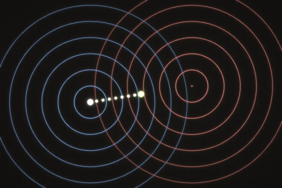 Fine-tuning seen in parameter space. Each step goes down the chat loss (coral rings) and so climbs the Shakespeare loss (blue rings), because the same parameters serve both. A lower learning rate or fewer steps stop the path closer to where it started.
To recap: fine-tuning at a lower learning rate moved the model toward chat replies, held-out ones included, and away from Shakespeare. It changed the form of the replies far more than their content, and its loss was the pretraining loss with a mask.
SFT still needs someone to write every ideal answer, and it never shows the model a worse one. The next lesson trains on comparisons between answers and on answers a program can check, and fine-tunes large models cheaply by training only a small change to each weight matrix.