Step against the gradient and repeat. Why that works, exactly how large a step can be before training blows up, why narrow valleys make it crawl, and how momentum speeds it up.
About 70 minutes
By the end you can
Explain from the linear approximation why a small step against the gradient lowers the loss.
Derive wk+1−w∗=(1−ηa)(wk−w∗) for a one-dimensional quadratic and read off the stable range 0<η<2/a.
Use the Hessian's eigenvalues to predict the learning-rate limit 2/λmax and the slowdown caused by a large condition number.
Explain what momentum changes, derive why no direction can shrink faster than β per step, and implement it.
You can now compute the gradient of a loss: the direction in which it climbs fastest. The algorithm that trains nearly every neural network, including the largest language models, is the natural next move. Take a small step the opposite way, recompute the gradient, and repeat:
w←w−η∇L(w).
The arrow means "replace w by". The number η (the Greek letter eta) is the learning rate: how far to step, as a multiple of the gradient. Everything interesting hides in the word "small". Too small and training wastes days of compute. Too large and the loss explodes.
This lesson works out exactly where the line is and why it sits there. First one step, with every number. Then one dimension, where everything can be solved by hand. Then many weights, where the shape of the valley matters. Finally momentum, the first fix. The next lesson moves to real data.
Why should a step against the gradient lower the loss at all? The forecast from the gradients lesson, L(w+h)≈L(w)+∇L(w)⋅h, answers it in two moves. Write g=∇L(w) for the gradient at the current weights. The step is h=−ηg.
Put the step into the forecast:
L(w−ηg)≈L(w)+g⋅(−ηg).
Pull the number −η out of the dot product, and use the fact that a vector dotted with itself is its squared length, g⋅g=∣g∣2:
L(w−ηg)≈L(w)−η∣g∣2.
Since ∣g∣2 is positive whenever the gradient is not zero, a small enough step lowers the loss, by about η∣g∣2. The forecast ignores curvature, and curvature is exactly what bites when η is large; the rest of the lesson measures it. When the gradient is zero the step is zero and descent stops. That happens at a minimum, but also at a maximum or at a saddle point, a point where the surface curves up in some directions and down in others.
A worked example in one dimension. Take the loss from the start of the module, L(w)=(w−3)2, whose minimum is at w=3. With one weight the gradient is the ordinary derivative, L′(w)=2(w−3). Use the learning rate η=0.1 and start at w0=0. One full step:
Loss at the start.L(0)=(0−3)2=9.
Slope at the start.L′(0)=2(0−3)=−6.
The step.−ηL′(0)=−0.1×(−6)=+0.6. The minus sign turns a negative slope into a step to the right, toward the minimum.
The new weight.w1=0+0.6=0.6, where L(0.6)=(0.6−3)2=(−2.4)2=5.76.
Compare with the forecast. The forecast drop is η∣g∣2=0.1×(−6)2=0.1×36=3.6. The real drop is 9−5.76=3.24, a little less, because the curve bends up away from its tangent.
The diagram draws that step on the curve, then three more, then what a much larger learning rate does. On screen are the pink loss curve L(w)=(w−3)2 with its minimum marked on the axis at w=3, and the current weight as a white dot on the curve. Beside it a table fills in one row per iterate k: the weight wk, its loss L (pink), the slope there (amber) and the step it produces (lime). Step through with Next.
Here are the first four iterates at η=0.1 in one table, with the distance still to go:
step k
wk
gradient 2(wk−3)
wk+1=wk−0.1×gradient
distance 3−wk
0
0
−6
0.6
3
1
0.6
−4.8
1.08
2.4
2
1.08
−3.84
1.464
1.92
3
1.464
−3.072
1.7712
1.536
The distance shrinks by the same factor at every step: 2.4/3=0.8, 1.92/2.4=0.8 and 1.536/1.92=0.8. At η=1.1 the distances were 3, 3.6, 4.32 and 5.184, each 1.2 times the one before, on alternating sides. Why 0.8, and why 1.2? The next section solves the one-dimensional case exactly.
Near its minimum, every smooth loss looks like a bowl. So working out what gradient descent does on the simplest bowl, exactly, tells you what it does near any minimum.
Take a quadratic with its minimum at w∗:
L(w)=2a(w−w∗)2,a>0.
Its derivative is L′(w)=2a×2(w−w∗)=a(w−w∗), and its second derivative is L′′(w)=a. So a is the curvature: how quickly the slope changes, or how sharply the bowl bends. Our example (w−3)2 is this bowl with w∗=3 and a=2, since (w−3)2=22(w−3)2.
Go slower: The error after one step, and after many
Step 1, write out the update. Gradient descent replaces wk by wk−ηL′(wk). Substitute L′(wk)=a(wk−w∗):
wk+1=wk−ηa(wk−w∗).
Step 2, subtract w∗ from both sides.
wk+1−w∗=(wk−w∗)−ηa(wk−w∗).
Step 3, factor out (wk−w∗).
wk+1−w∗=(1−ηa)(wk−w∗).
Step 4, repeat. Call the error ek=wk−w∗. Every step multiplies it by the same number, ek+1=(1−ηa)ek, so after k steps
ek=(1−ηa)ke0.
Step 5, when does it shrink? Powers of a number go to zero exactly when the number's size is below 1: ∣1−ηa∣<1. That means −1<1−ηa<1, two inequalities to solve one at a time.
The right one, 1−ηa<1: subtract 1 to get −ηa<0, so ηa>0, and since a>0, η>0.
The left one, −1<1−ηa: add ηa+1 to both sides to get ηa<2, so η<2/a.
Together:
0<η<a2.
For our example the factor is 1−ηa=1−0.1×2=0.8: the factor in the table. With η=1.1 it is 1−1.1×2=−1.2. The minus sign is the jump to the other side, and the size 1.2 is the growth. The limit is 2/a=2/2=1, and 1.1 is above it.
Here is every regime, for a bowl with curvature a=4, L(w)=2(w−1)2:
learning rate η
factor 1−4η
what happens
0.1
0.6
smooth approach from one side
0.25=1/a
0
lands on the minimum in one step
0.4
−0.6
overshoots, alternates sides, still converges
0.5=2/a
−1
bounces between two points forever
0.6
−1.4
overshoots further every step: diverges
A negative factor means the step jumps past the minimum to the other side. Its size decides whether each jump lands closer or farther. This is the repeated multiplication from module 4 in its simplest form: a number with size below 1, raised to higher and higher powers, dies away, and one above 1 explodes.
The widget runs the same rule on a round bowl, L=x2+y2, seen from above as a contour map: pink lines of equal loss, shading that darkens toward the bottom, and a lime cross at the minimum. It has two weights, but it curves the same way in every direction, with curvature 2, exactly like (w−3)2, so each step multiplies the distance to the minimum by 1−2η. The blue dot is the start, (−2.6,1.8); the path collects a white dot per step; the amber arrow shows where the next step goes. Among the controls, a stability panel gives the factor per step, a coral tick under the learning-rate slider marks the limit, and a chart at the bottom plots the loss after each step.
Now run three steps by hand on a sharper bowl, and find the learning rate at which it breaks.
On paperThree steps by hand, and the breaking point
Run gradient descent on L(w)=3(w−2)2 from w0=0 with learning rate η=0.1.
Compute w1, w2 and w3, showing the gradient at each step.
Write L in the form 2a(w−w∗)2 and find the factor 1−ηa. Check that the distance to the minimum shrinks by that factor.
Find the learning rate at and above which gradient descent no longer converges on this loss. What happens at η=0.3?
To check your work, enter w1, w2, w3 and then the threshold learning rate, in that order, as decimals (you may enter the threshold as a fraction, such as 2/5).
Work it on real paper: writing each step is the point. Then check your final answer here and compare your working with the walk-through.
w₁, w₂, w₃, then the threshold
One entry per box, top to bottom. 0.25, -2, 3/4 and sqrt(2) all work. Enter moves to the next empty box and checks once all are filled.
With one weight, one number described the bowl's curvature. With many weights, curvature depends on direction: a valley can be steep across and nearly flat along its floor. We need an object that records curvature in every direction.
That object is the Hessian, the matrix of second derivatives:
Hij=∂wi∂wj∂2L,
meaning: differentiate L with respect to wj, then differentiate the result with respect to wi. Equivalently, the Hessian is the Jacobian of the gradient. For the smooth functions in this course the order of the two derivatives does not matter, so Hij=Hji and the Hessian is symmetric.
An example: L(w)=21(w12+10w22).
The gradient.∂w1∂L=21×2w1=w1 and ∂w2∂L=21×10×2w2=10w2, so ∇L=(w1,10w2).
Differentiate each entry again.w1 has partials 1 (by w1) and 0 (by w2); 10w2 has partials 0 and 10.
The Hessian.H=[10010]: this valley is ten times more curved across w2 than along w1.
Why study quadratic bowls? Recall Taylor's formula from derivatives by experiment: value, plus slope times the step, plus 21 curvature times the step squared. In many dimensions the gradient plays the slope and the Hessian plays the curvature. At a minimum w∗ the gradient is zero, so the formula has no first-order term and starts with the curvature term:
L(w)≈L(w∗)+21(w−w∗)⊤H(w−w∗),
with H the Hessian at w∗. Near any minimum, a smooth loss looks like a quadratic bowl, so what gradient descent does on bowls is what it does near minima. On this bowl the gradient is H(w−w∗), by the quadratic-form rule from the gradients lesson (the 21 cancels the 2). For the example, with w∗=0, that is (w1,10w2), as we found.
Go slower: Gradient descent on a bowl, one eigen-direction at a time
Step 1, the error update. Let ek=wk−w∗. The gradient at wk is Hek, so the update is wk+1=wk−ηHek. Subtract w∗ from both sides:
ek+1=ek−ηHek=(I−ηH)ek.
So the error is multiplied by the same matrix every step, and ek=(I−ηH)ke0.
Step 2, use the eigenvectors.H is symmetric, so (module 4) it has perpendicular unit eigenvectors v1,…,vn with real eigenvalues λ1,…,λn. Write the starting error in that basis: e0=c1v1+⋯+cnvn.
Step 3, each direction on its own. Since Hvi=λivi, we get (I−ηH)vi=vi−ηλivi=(1−ηλi)vi. Applying the matrix k times multiplies each piece by its own factor k times:
ek=(1−ηλ1)kc1v1+⋯+(1−ηλn)kcnvn.
Each eigen-direction is a separate one-dimensional problem with curvature λi.
Step 4, the limit. Every piece shrinks only if ∣1−ηλi∣<1 for every i, which means η<2/λi for all of them, and the binding one is the largest eigenvalue: η<2/λmax.
Step 5, the best single learning rate. The slowest piece decides the pace, so choose η to make the worst factor as small as possible. As η grows, ∣1−ηλmin∣ shrinks while ∣1−ηλmax∣ eventually grows. The best balance is where the two sizes are equal. At that rate the flat direction's factor 1−ηλmin is still positive, while the steep direction's factor is negative, with size ηλmax−1. So the balance reads 1−ηλmin=ηλmax−1. Add 1+ηλmin to both sides: 2=η(λmin+λmax), so η=λmin+λmax2.
Step 6, the factor at that rate. Substitute into 1−ηλmin: 1−λmin+λmax2λmin=λmax+λminλmax−λmin. Divide the top and bottom by λmin to get κ+1κ−1, where κ=λmax/λmin.
So far. The Hessian records curvature in every direction. Along each of its eigenvectors, gradient descent is the one-dimensional problem again, with curvature λi and factor 1−ηλi per step.
Two numbers fall out of the eigen-direction picture, and together they explain why training can be unstable and slow at the same time.
The learning-rate limit2/λmax, set by the steepest direction.
The condition numberκ=λmax/λmin. When it is large, any learning rate small enough for the steep direction is far too small for the flat one. Even the best single rate shrinks the error only by a factor of κ+1κ−1 per step, which is close to 1.
Take the valley H=diag(1,10) from above, with κ=10/1=10.
The limit.η<2/λmax=2/10=0.2.
A rate near the limit, η=0.18. The factors are 1−0.18×1=0.82 along w1 and 1−0.18×10=−0.8 across w2. The w2 coordinate flips sign at every step, so the path zig-zags across the valley while creeping along it.
The best rate.η=1+102=112≈0.182, with factor 10+110−1=119≈0.818 in both directions. Shrinking the error a thousandfold takes 35 steps, since (9/11)35<0.001<(9/11)34.
Worse conditioning. With κ=100 the best factor is 10199≈0.980, and the same thousandfold shrink takes 346 steps.
Ten times worse conditioning, ten times more steps. The code runs the κ=10 valley from (1,1) at three learning rates and plots the loss:
⌘+Enter runs · edit freelyPython sleeps until you run code
At η=0.05 both coordinates shrink smoothly but w1 crawls (1, 0.95, 0.902, 0.857). At 0.18 the second coordinate alternates sign (1, −0.8, 0.64, −0.512: the zig-zag) and the loss falls fast. At 0.21, just past the limit, the second coordinate grows by a factor of 1.1 per step (1, −1.1, 1.21, −1.331) and the loss explodes.
The widget runs this same valley, L=21x2+5y2, whose Hessian is diag(1,10). The steep direction is y, across the valley; the flat one is x, along its floor. The run starts at (−2.8,1.6) with η=0.05. The stability panel lists each curvature λ with its factor per step, and the coral tick under the learning-rate slider marks the limit 0.2.
This is why learning rates are tuned by experiment when you train networks in module 6, and why the optimizers used to train LSTMs in module 8 rescale different directions differently. The eigenvalues are not known in advance for a real network, and they change during training, but the logic is the same: the sharpest direction caps the step, and the flattest direction sets the pace.
So far. The largest curvature caps the learning rate at 2/λmax. The smallest curvature then sets the pace, and their ratio κ says how slow even the best single learning rate must be.
Find a learning-rate limit from a Hessian you compute yourself.
Work it outThe largest safe learning rate
The loss is L(w)=1.5w12+w1w2+1.5w22. Find its Hessian, then the learning rate at which gradient descent stops converging. Enter that learning rate as a decimal.
largest stable η
Type a number: 0.25, -2, 3/4 and sqrt(2) all work. Enter checks.
Now run the reasoning backwards: from three training runs, bracket the curvature.
Quick checkRead the curvature off three runs
You train the same model three times with full-batch gradient descent, starting close to a minimum. With η=0.01 the loss falls slowly and steadily. With η=0.1 it falls fast. With η=0.3 it grows by roughly the same factor every step. Treating the loss near the minimum as a quadratic bowl, what can you conclude about the largest Hessian eigenvalue λmax?
The zig-zag suggests its own fix. Across the valley, successive gradients point in opposite directions. Along the valley floor, they point the same way every time. If we averaged recent gradients, the across-valley parts would cancel and the along-valley parts would add up.
That is momentum. Keep a running "velocity" v and step along it:
v←βv+∇L(w),w←w−ηv,
with v starting at zero and β between 0 and 1, often 0.9. Write gk for the gradient at step k and unroll the first three velocities:
v1=β⋅0+g1=g1,
v2=βv1+g2=g2+βg1,
v3=βv2+g3=g3+βg2+β2g1.
The pattern continues: the velocity is a weighted sum of all past gradients, vk=gk+βgk−1+β2gk−2+⋯, with weights fading geometrically. Two consequences:
Where the gradient keeps the same value g, the velocity grows toward g(1+β+β2+⋯)=g/(1−β), the sum of a geometric series. With β=0.9 that is g/0.1=10g: a step ten times larger along steady directions.
Where the gradient alternates sign, g,−g,g,…, successive terms largely cancel. The velocity settles at g/(1+β) in size, about 0.53g with β=0.9, so the zig-zag is damped instead of amplified.
The picture behind the name is a heavy ball rolling down the valley: its inertia carries it along the floor and smooths out the side-to-side bouncing.
Momentum: the side-to-side pushes cancel, the steady pull along the floor adds up.
The method is often called Polyak's heavy-ball method, after Boris Polyak, who analyzed it in 1964. On the valley H=diag(1,100), starting at (1,1) with η=0.01, plain gradient descent needs 1,375 steps to get within 10−6 of the minimum; with momentum β=0.9 and the same η it needs 264. The momentum coefficient is itself a knob, not a free lunch: on the same problem, β=0.5 takes 671 steps, 0.8 takes 192 and 0.95 takes 498, because too much momentum overshoots and oscillates along the floor.
Why does momentum help so much here, and why does more momentum stop helping? Along each eigen-direction of the Hessian, momentum turns the one-step error rule of the last section into a two-step rule, and that rule has a simple bound: a limit on how fast any direction can shrink.
Go slower: Momentum along one eigen-direction
Take one eigen-direction with curvature λ. Let ek be the error along it (the distance to the minimum, with a sign) and vk the velocity along it, starting at v0=0. The gradient along it is λek, so the two updates are
vk+1=βvk+λek,ek+1=ek−ηvk+1.
Step 1, multiply the velocity update by η.
ηvk+1=βηvk+ηλek.
Step 2, remove the velocity. The second update says ηvk+1=ek−ek+1, and one step earlier ηvk=ek−1−ek. Substitute both:
ek−ek+1=β(ek−1−ek)+ηλek.
Step 3, solve for the new error. Move ek+1 to the left side alone and collect the ek terms:
ek+1=(1+β−ηλ)ek−βek−1.
Each error now depends on the two before it. With β=0 this is the old rule ek+1=(1−ηλ)ek.
Step 4, look for a constant factor. Try ek=rk, an error multiplied by the same number r every step. Substitute: rk+1=(1+β−ηλ)rk−βrk−1. Divide by rk−1 and move everything to one side:
r2−(1+β−ηλ)r+β=0.
This quadratic has two roots r1 and r2, and the error is a mix of r1k and r2k. The root with the larger size sets the pace. When the roots are complex, the error oscillates as it shrinks: the overshooting you see along the valley floor.
Step 5, a bound on the speed. A quadratic r2+br+c with roots r1,r2 factors as (r−r1)(r−r2)=r2−(r1+r2)r+r1r2, so the product of its roots is its constant term c. Here r1r2=β, so the sizes multiply to ∣r1∣∣r2∣=β. They cannot both be below β, or their product would be below β×β=β. So the larger root has size at least β, whatever η and λ are. With β=0.9, no direction can shrink faster than 0.9≈0.949 per step.
Step 6, the stability limit. For a tiny η both roots lie between −1 and 1 (they are close to 1 and to β), and as η grows they move continuously. Complex roots have size exactly β<1, so they cannot escape. Real roots can only escape by passing through r=1 or r=−1. Putting r=1 in the quadratic gives 1−1−β+ηλ+β=ηλ=0, which never happens. Putting r=−1 gives 1+1+β−ηλ+β=2(1+β)−ηλ=0. So descent with momentum is stable exactly when ηλ<2(1+β): momentum raises the limit from 2/λmax to 2(1+β)/λmax.
Now the step counts make sense. On diag(1,100) with η=0.01, plain descent's flat direction shrinks by 1−0.01×1=0.99 per step, and 0.991375≈10−6. Momentum 0.9 brings every direction down to the bound 0.9≈0.949, and 0.949264≈10−6. The best β balances two effects: large enough to speed up the flat direction, small enough to keep the bound β low. At β=0.5 the flat direction still shrinks only by about 0.980 per step (671 steps); at 0.8 its factor is about 0.927 (192 steps); at 0.95 the bound has risen to 0.95≈0.975 (498 steps). And on a milder valley, where plain descent already beats 0.949 per step, momentum 0.9 makes things worse: a milder valley wants a smaller β.
The widget runs the valley from before, L=21x2+5y2, with the same learning rate, 0.05, now with momentum β=0.6. The formula panel shows both updates with live numbers, the velocity first. The stability panel shows each direction's factor, and the coral tick marks the raised limit 2(1+β)/λmax.
In short. Momentum adds a fraction β of the last step to each new one. Steady directions speed up by up to 1/(1−β), alternating ones are damped, and no direction can shrink faster than β per step, so the best β depends on how badly conditioned the valley is.
Now build both methods, check the stability limit, and reproduce the step counts above.
Code itGradient descent and momentum on a bowl
Explore gradient descent on the bowl L(w)=21(w−w∗)⊤H(w−w∗), whose gradient is H(w−w∗).
gd_path(H, w_star, w0, lr, steps): every iterate, start included, as an array of shape (steps + 1, d).
max_stable_lr(H): the limit 2/λmax.
momentum_path(H, w_star, w0, lr, beta, steps): the same with momentum, v←βv+∇L and w←w−ηv, starting from v=0.
steps_to_reach(path, w_star, tol): the first index whose distance to w∗ is below tol, or None.
The code at the bottom races plain descent against momentum on the valley diag(1,100). It should reproduce the lesson's 1,375 and 264 steps.
⌘+Enter runsPython sleeps until you run code
Write your code where the starter says raise NotImplementedError, then press Run tests. Each check says what it expects.
Everything in this lesson used the exact gradient of a loss written as one short formula. A real training loss is an average over millions of examples, and computing its exact gradient on every step is too expensive. The next lesson estimates it from small random batches, meets Adam, and fits a real model both exactly and by descent.


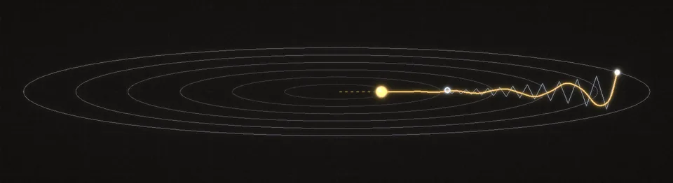 Momentum: the side-to-side pushes cancel, the steady pull along the floor adds up.