
Lesson 1 of 6
Derivatives as zoom
Zoom in far enough on a smooth curve and it becomes a straight line. The slope of that line is the derivative, and the approximation it gives is the idea every training algorithm runs on.
Explain the derivative as the slope of the best local straight-line approximation, and use that approximation to estimate values.
Apply the sum, power, product and chain rules, and say why each one holds.
Derive and state the derivatives of , , and ReLU.
Explain why saturated sigmoid and tanh units pass almost no gradient back.

You are training a model with a single weight . The loss is , but pretend you cannot see that formula: all you can do is set the weight, run the model and read the loss. At the loss is . Nudge the weight to and the loss becomes . The loss changed by while the weight changed by , so it moved at a rate of : about units of loss per unit of weight.
That rate is the derivative, and it answers the one question training asks over and over: if I move this weight a little, what happens to the loss? A negative rate says "increase the weight and the loss goes down". A language model asks that question for billions of weights at once, on every training step. Modules 1 to 4 built the linear algebra of what a network computes; this module adds the calculus of how to change it, and builds the tools to answer that question for vectors and matrices. This lesson starts with one input and one output, because every later idea is this one wearing more dimensions.
The lesson builds the idea in four steps: the picture (zoom in until a curve is a line), what that line predicts, the rules that compute derivatives without any zooming, and the derivatives of the functions networks are made of. The next lesson measures derivatives by experiment, so you can check your formulas.
Zoom in until the curve is a line
A curve is hard to reason about, because its steepness keeps changing. A straight line is easy: it changes at one fixed rate everywhere. The first idea of calculus is that a smooth curve, looked at closely enough around one point, is a straight line.
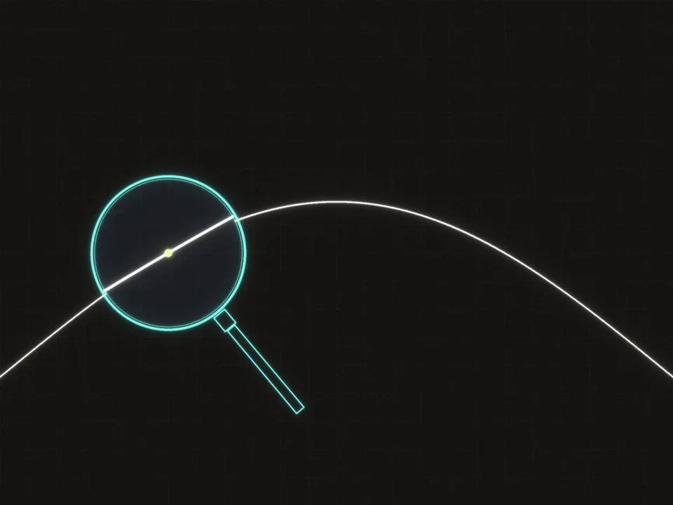 Up close, a smooth curve cannot be told apart from a straight line.
The widget below lets you test that claim on . The white curve is , the blue dot is the point on it, and the amber line is the straight line through that point with the curve's steepness there. The readouts give , the height , the slope of the amber line, and the largest gap between the curve and the line anywhere in view.
The line the curve turns into is the tangent line, and its slope is the derivative of at , written and read "f prime of x". For at it is , the number in the widget.
To pin the slope down with numbers, take a second point a small step to the right of the first. The straight line through and is called a secant. Its slope is rise over run: the change in output, , divided by the change in input, . Now let the second point slide toward the first:
Read as "the value this fraction settles on as gets closer and closer to zero". We cannot set directly, because the fraction would become ; the limit asks where the fraction is heading instead.
A worked example: at , where . Work out the secant's slope one move at a time.
- Expand the square: .
- Subtract to get the rise: .
- Divide by the run to get the slope: .
With the secant's slope is ; with it is . As shrinks the slope settles on , so : near , the output changes about 6 times as fast as the input.
The tangent line predicts nearby values
A slope is useful because it predicts. If you know a function's value at one point and its slope there, you can estimate its value a small step away without computing the function again. Training does exactly this: it uses the slope at the current weights to predict which small change lowers the loss.
The prediction comes straight out of the definition, in three moves.
-
For a small but nonzero , the fraction is close to the number it settles on:
-
Multiply both sides by :
-
Add to both sides:
In words: start at the height and climb for every unit of step. That is the tangent line, used as a forecast.
How good is the forecast? For at the line predicts , and the truth is , so the error is exactly .
| step | true | line | error |
|---|---|---|---|
Shrink the step 10 times and the error shrinks 100 times. That is the precise sense in which the tangent is the best line through the point. Any other line through , with some slope , predicts . Its error is the truth minus the prediction:
For a small the term is far bigger than , so this error shrinks only as fast as : halve the step and the error only halves. The slope is the one choice that removes that term, leaving an error of , which shrinks faster than the step itself: the error divided by the step, , goes to zero.
That property is the definition worth keeping. Written out, is differentiable at when some number makes
Here is the leftover error. This version generalizes without change: in the gradients lesson becomes a vector, and in Jacobians and the chain rule a matrix.
The same pattern holds for curves that are not polynomials. The code below measures the error of the tangent line for at at three step sizes, and divides each error by to test whether it shrinks like :
The error falls a hundredfold per row, and the ratio settles near ; the next lesson explains exactly where that constant comes from.
A derivative has units: output per unit of input. That makes it a sensitivity you can use for quick estimates. Take , whose derivative is (the next section shows why), and estimate from the nearby point , where the square root is easy.
- The value there: .
- The slope there: .
- The step: .
- The forecast: .
The true value is to five decimal places, so the forecast is off by about .
So far. Zoom in on a smooth curve and it becomes a straight line, its tangent. The tangent's slope is the derivative. The tangent predicts nearby values, , with an error that shrinks faster than the step.
Now make a forecast of your own. The next exercise uses the tangent at to estimate a cube just below it.
The derivative of is (the power rule, in the next section). Use the tangent line at to estimate . Enter the estimate, not the exact value, as a decimal.
Type a number: 0.25, -2, 3/4 and sqrt(2) all work. Enter checks.
The rules, each with a reason
Computing a limit for every function would be slow. A handful of rules build every derivative you need from a few known ones. Each rule has a one-line reason, and the reasons matter more than the rules: they are the same reasons in many dimensions, in the next two lessons.
Sums and constant multiples. for constants and . Near , and each act like lines, so does too, and slopes of lines scale and add. Differentiation is linear, just as the dot product was in module 1.
Powers. . Take and multiply out the nudged value:
The first term is the old value and the second is times the step, so is the slope. The last two terms contain or and vanish faster than , so they do not change the slope. For any whole number the same happens. is brackets multiplied together, and multiplying out means picking or from each bracket in every possible way and adding up the products. Picking every time gives . Picking from exactly one bracket and from the other gives , and there are brackets to pick that from, so together these give . Every other way picks at least twice, giving terms with or higher powers. So the slope of is . The rule holds for any real exponent (the logarithm below shows why): has derivative , and has derivative .
Products. . Picture as the area of a rectangle with sides and . Nudge by : the sides grow to about and . Multiply out the new area:
The first term is the old area. The next two are thin strips along two sides of the rectangle: is a strip wide running along the side of length , and is a strip tall running along the side of length . The last is a tiny corner, by , that vanishes faster than . So the area grows by about , and its slope is .
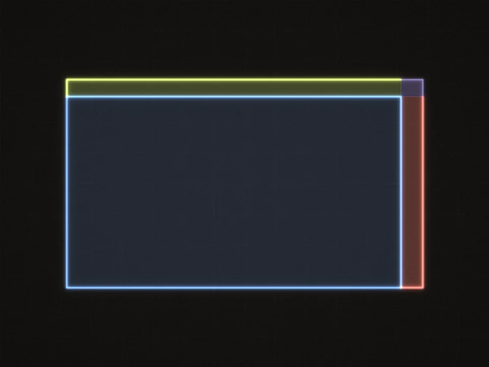 A product grows by two thin strips, plus a corner too small to matter.
Composition (the chain rule). Write for "apply , then ", the function . Then .
The chain rule is the one that matters most, and the zoom picture explains it. Near , the inner function acts like multiplication by its slope: a small nudge at becomes a nudge of about at . Near , the outer function acts like multiplication by its own slope there, . Two stretches in a row multiply: if stretches small nudges by 3 and stretches them by 8, a nudge that passes through both is stretched by 24.
Go slower: The chain rule from two linear approximations
Let be the point where receives its input.
Step 1, the inner function. For a small step , , where is the nudge that arrives at .
Step 2, the outer function. For the small step , .
Step 3, substitute. Replace by and by :
Step 4, read off the slope. This has the form "value plus slope times ", so the slope of at is .
Two errors were dropped along the way: the inner approximation's and the outer one's. Each shrinks faster than its own step, and the step that reaches is at most a fixed multiple of , so the combined error also shrinks faster than . That is what turns the picture into a proof.
Notice where is evaluated: at , where actually receives its input, not at . Getting this wrong is the most common chain-rule slip.
A worked example: at .
- Split it. The inner function is and the outer function is .
- Find where the outer function receives its input. At , .
- Inner slope. .
- Outer slope, at . .
- Multiply. .
Check by expanding first: , whose derivative is , and .
The notation ("the derivative of with respect to ") makes the rule look like fractions cancelling: . That is a good memory aid, not a proof.
This rule is the seed of backpropagation. A neural network is a long composition of functions, so its derivative is a long product of local slopes. In the Jacobians lesson the slopes become Jacobian matrices and the product becomes matrix multiplication, the same composition-as-multiplication you met in module 2. In module 6 that product is backprop.
The four rules in one line each. Slopes of sums add. has slope . A product's slope is two strips, . A composition's slope is the product of the slopes, with the outer slope taken where the outer function receives its input.
Practice the chain rule on two composites. The second has three layers, which is the shape of every network: find each layer's slope where that layer receives its input, then multiply.
Differentiate each function with the chain rule. Name the inner and outer functions, find each slope where its function receives its input, then evaluate at the given point.
- at .
- at . This one has three layers: , then , then .
To check your work, enter and then , both whole numbers.
Work it on real paper: writing each step is the point. Then check your final answer here and compare your working with the walk-through.
One entry per box, top to bottom. 0.25, -2, 3/4 and sqrt(2) all work. Enter moves to the next empty box and checks once all are filled.
The derivatives a network needs
A network is assembled from a few functions: exponentials and logarithms inside its losses, and squashing functions between its layers. Here are their derivatives, each built from the rules above.
The exponential. is its own derivative. Here is why, one move at a time.
- The exponent rule splits the nudged value: .
- The number is exactly the base whose graph crosses the vertical axis with slope 1. So the tangent line of at starts at height and climbs with slope 1, and for small , . Check: , which is plus a leftover of about .
- Substitute: .
- This has the form "value plus slope times ", so the slope is .
The chain rule with inner function (slope ) gives , which we need in a moment.
The logarithm. The natural logarithm undoes the exponential: for . Differentiate both sides of that equation.
- The left side is a composition: outer function (slope ), inner function . The chain rule gives . The right side, , has slope .
- Replace by : the equation reads .
- Divide by : .
Logarithms appear in every loss you will train with, starting with cross-entropy in module 6.
The logarithm also settles the power rule for any real exponent . For , write . The outer function has slope and the inner function has slope , so the chain rule gives . With this is the square root's slope, , used for above.
The sigmoid. squashes any number into the interval from 0 to 1. (The letter has already named a standard deviation in module 0 and the singular values in module 4; used as a function without a subscript, as in , it is always the sigmoid.) It is the output of logistic regression and the gate in every LSTM. Its derivative has a compact form:
Go slower: Deriving the sigmoid's derivative
Step 1, rewrite as a power. . The outer function is and the inner function is .
Step 2, the two slopes. The outer slope is (power rule). The inner slope is , using the slope of from above.
Step 3, multiply (chain rule). Evaluate the outer slope at :
Step 4, tidy up. The two minus signs cancel, and a power of means one over the square:
Step 5, split into two factors.
The first factor is .
Step 6, recognize the second factor. Add and subtract 1 in its numerator, then split the fraction:
Step 7, combine. .
Two consequences. First, once the forward pass has computed , the derivative costs one multiplication, . Backprop reuses forward values like this all the time. Second, the slope is never larger than . The product is zero at and at and is a downward parabola in between, so its peak sits halfway, at , where it equals . The sigmoid outputs at , because . So everywhere.
The hyperbolic tangent. squashes into the interval from to and is centered at zero. It is the nonlinearity of plain recurrent networks and appears twice inside an LSTM. Its derivative is
which is at . Again the forward value is all you need: if , the slope is .
Go slower: Why tanh' = 1 - tanh²
Step 1, tanh is a stretched sigmoid. Start from , write the sigmoid out, and put everything over one denominator:
Multiply top and bottom by to get .
Step 2, differentiate with the chain rule. In the constant has slope 0 and the factor 2 stays in front. The piece is the sigmoid of the inner function , whose slope is 2, so its slope is . Together:
Step 3, use the sigmoid's rule. Write . Then , so .
Step 4, compare with . Since , expand the square and subtract:
The two agree, so .
ReLU. is the default activation of deep feed-forward networks. Its derivative is for and for . At the graph has a corner and no single tangent line: the slope from the left is 0 and from the right is 1. Code must pick a value there, and frameworks pick one of the two (commonly 0). It rarely matters, because an input lands on exactly zero only rarely. What does matter: a unit whose input is negative passes back no gradient at all.
Now compare the three side by side. The widget answers one question: for which inputs does each unit pass a gradient back, and for which does it all but block it? On screen are the sigmoid (teal), tanh (violet) and ReLU (coral), each with its slope drawn as a dashed curve of the same color. A dashed blue line marks the input , moved by the handle at the bottom, by tapping the plot or with the slider. The table lists each function's value and slope at . The thick curve is the focused function, and hatched bands mark where its slope is smaller than .
Here are the same quantities at three inputs, to more digits:
Once the input is more than a few units from zero, both curves are nearly flat and their slopes are close to zero. The unit is saturated. Combine that with the chain rule. Apply the sigmoid ten times in a row, , and the chain rule gives a product of ten slopes, each at most . Even in the best case the product is at most , the slope¹⁰ readout above. In a real network, weights multiply into the chain as well and can partly compensate, but the tendency is real: the signal telling early layers how to change fades as it passes back through saturated units. This is the vanishing-gradient problem in its smallest form. It returns in module 7, where a recurrent network multiplies such factors once per time step, and the LSTM's cell state in module 8 is the fix.
So far. is its own slope and has slope . The sigmoid's slope is , at most ; tanh's is , at most ; ReLU's is or . All three slopes come from the forward output alone, and the two squashing functions' slopes fade toward zero for large inputs.
Derive the sigmoid's derivative yourself now, without looking back, and then evaluate it at a point where the numbers come out as simple fractions.
Without looking back, derive for . Then use it:
- Check that , then compute .
- Check that , then compute from .
To check your work, enter and then , as fractions (such as 5/8) or decimals.
Work it on real paper: writing each step is the point. Then check your final answer here and compare your working with the walk-through.
One entry per box, top to bottom. 0.25, -2, 3/4 and sqrt(2) all work. Enter moves to the next empty box and checks once all are filled.
Next, use those slopes to compare how much gradient four different units pass back.
Four units each receive an upstream gradient of from the layer above. By the chain rule, each passes back times its own slope at its input. Which one passes back the least?
Choose one answer, then check.
Then put the chain rule and the sigmoid's slope together to explain a classic training failure.
A colleague builds a 10-layer network with a sigmoid after every layer. During training the last layers learn well, but the first layers barely change. Explain why, using the chain rule and the sigmoid's derivative, and suggest what to change.
Saved in this browser as you type.
For more practice with the rules and these derivatives, work through a few generated problems. Each comes with a worked solution.
Let . Find .
Type a number: 0.25, -2, 3/4 and sqrt(2) all work. Enter checks.
You now have derivatives by formula. The next lesson measures them by experiment instead, which is how every formula in this course gets checked.