
Lesson 1 of 6
The cell state and its gates
An LSTM adds a second memory, the cell state, that is scaled and added to instead of being rewritten through a matrix at every step. Four small gates decide what to erase, what to write and what to show.
Explain why a memory that is added to can carry a signal across many steps, and name the three problems that the forget, input and output gates fix.
Write the LSTM equations with the shape of every vector and matrix, both in column form and in the stacked row form used in code.
Compute one LSTM step by hand.
Say what each of the four gates does, and predict how changing one of them changes the cell's behavior over several steps.
Implement a vectorized LSTM step with all four gates in one matrix product.

In module 7 a plain recurrent network failed a simple memory test. It sees one symbol, then a long stretch of unrelated tokens, then a cue, and it has to answer with the first symbol. With a short gap it learns the task. With a long gap it stays at chance, and training longer moves the limit out only slowly.
The reason was in the backward pass. The gradient that would teach the network to store the first symbol has to travel back to the first step, and on the way it is multiplied by one Jacobian per step. If each multiplication shrinks it by a factor of 0.8, then after 10 steps of it is left, after 20 steps , and after 40 steps . The network never finds out that the first symbol mattered.
This lesson builds the fix from one question: what would a memory have to look like for a signal to cross 40 steps intact? The answer is the cell state of a long short-term memory network, or LSTM. The name says what it is for: a short-term memory (the network's changing activations, as opposed to its weights) that can last a long time. Here we build the cell going forward: what it computes, what each part is for, and how to code it. The next lesson follows a gradient backwards through it.
A memory that is added to
To see what shape a good memory needs, start from what goes wrong with the plain RNN's. It rewrites its whole state at every step:
Here is the input at step , is the hidden state, and are weight matrices and is a bias vector. Even when the network wants to keep one number exactly as it is, that number goes through the matrix and the squashing function at every step. Keeping it intact for 40 steps would need to leave it alone and the tanh to stay in its straight middle part, while the same matrix is also doing all of the network's other work.
Now try the simplest memory that does keep things: an accumulator. Call the memory and let the network add something to it at every step:
where is whatever the network computes to add at step . Follow the direct route from the old memory to the new one, with held fixed. Look at one entry first: . If goes up by a small amount, goes up by exactly the same amount, so the slope is . Entry of does not depend on any other entry of , so all the other slopes are 0. Collect these slopes into the Jacobian of module 5 (row , column holds ) and you get the identity matrix: . Going backwards, whatever gradient arrives at is multiplied by , so it reaches unchanged, and after 40 such steps it reaches unchanged too. That is exactly the property we asked for. The first LSTM, published in 1997, used this idea for its memory, and its authors called the path the constant error carousel: an error signal can go round it for as long as needed without shrinking or growing.
A pure accumulator has three problems, and each one becomes a gate.
- It can never erase. Once something is added it stays forever, and the sum can grow without limit. Fix: multiply the old memory by a number between 0 and 1 before adding. That number is the forget gate.
- It adds at every step, including junk. Fix: multiply what is written by a number between 0 and 1, so the network can decide when to write. That is the input gate.
- Everything stored is always visible to the rest of the network, even when it is not relevant yet. Fix: multiply what is shown by a number between 0 and 1. That is the output gate.
A small example shows why the second gate matters. Say one unit should remember a seen at step 1, and the next four steps would add noise of , , and . The accumulator adds everything: , so the noise has corrupted the memory by . Now put an input gate of 1 on step 1 and 0.05 on the noisy steps. The noise adds up to as before, but only of it gets in, and the memory ends at .
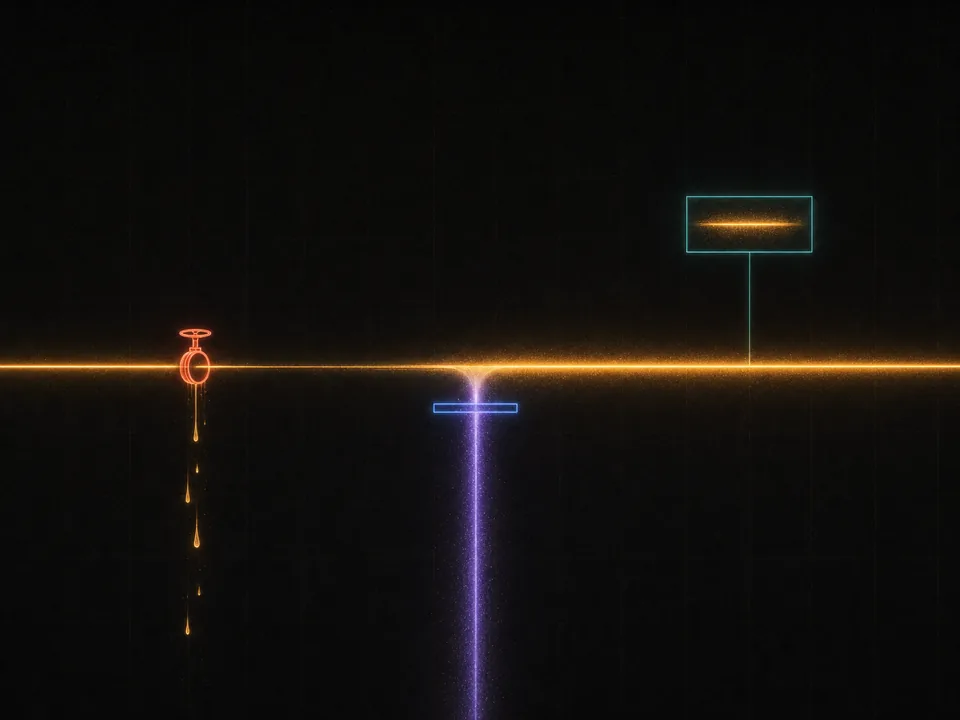 The cell state as a line that carries memory forward. First a valve decides how much stays, then a gate decides how much new content is added, and a window shows a squashed copy without removing anything.
To recap: the plain RNN pushes its memory through a matrix and a tanh at every step. An accumulator only adds to its memory, so a signal passes through it untouched, but it can neither erase, nor refuse to write, nor hide. The LSTM keeps the adding and puts a gate on each of those three jobs.
The full cell, with shapes
Before the equations, the question is what exactly gets written, kept and shown. One more piece completes the cell: the content that gets written, which the list above called "what is written", is computed by a fourth block, the candidate . It uses tanh, so it lies between and , and the input gate scales it before it is added.
The widget below is one LSTM cell with a single unit, so every quantity on it is one number. It answers one question: what does each gate do to the memory, and what does it do to the output? The thick amber line along the top is the memory: comes in on the left and leaves on the right. The four blocks are the forget gate (coral), the input gate (blue), the candidate (violet) and the output gate (teal), each filled to its current value. The input (white) and the previous output (lime) run along the bottom and feed every block, and the output leaves on the right. Each gate adds up a weight times , a weight times and a bias , then squashes the sum, so raising a gate's bias opens it further; the sliders set these weights and biases, one gate at a time. The readouts give , , the kept part (forget gate times ) and the written part (input gate times candidate). It starts at , and , with the widget's own weights, and the formulas beside the figure show every value.
Now the equations. The LSTM keeps two vectors from step to step: the cell state (the memory) and the hidden state (the output, which is also fed back in). At step it reads the input and the previous output , and computes four vectors:
Then it updates the memory and computes the output:
The symbol is the sigmoid , applied to every entry, and is the elementwise product: multiply matching entries. Many sources write the candidate as instead of ; it is the same vector. Each block has its own on the input and its own on the previous output, a common naming for LSTMs: they play the roles of the plain RNN's and . (Module 4 happened to use these two letters the other way round; in this module is always a weight on the previous output.)
The shapes, with input size and hidden size :
| Symbol | Shape | What it is |
|---|---|---|
| the input at step | ||
| previous and new output | ||
| previous and new cell state | ||
| weights on the input | ||
| weights on the previous output | ||
| biases | ||
| gates and candidate |
Check one line: is times , a vector of length ; is times , also length ; add (length ) and squash, and has length . Every gate has one entry per unit. Unit has its own forget value , its own input value and its own output value , and the products act entry by entry. So an LSTM layer is registers side by side. They interact only through , which every gate reads in full.
Three design choices are worth a sentence each.
- Gates use the sigmoid because they multiply: a gate value is a fraction, and the sigmoid's range from 0 to 1 is exactly the range of fractions.
- The candidate uses tanh because it is content, and content needs a sign. Its range from to keeps each write bounded, and it is centered on zero.
- The output applies tanh to the cell state because itself is not bounded. Repeated writes can push it well past 1 (the lesson after next uses this to count), so it is squashed back into before it is shown.
In short: three sigmoid gates and one tanh candidate, all computed from and ; the memory keeps a gated part of itself and adds a gated candidate; the output is a gated, squashed view of the memory.
One step by hand
Every later lesson in this module works with numbers like these, so it is worth doing one step completely. Take a single unit (), so every weight is a number. Write for the weight on , for the weight on and for the bias:
| (times ) | (times ) | ||
|---|---|---|---|
| forget | 1 | 2 | 0 |
| input | 2 | ||
| candidate | 1 | 0 | 0 |
| output | 2 |
The cell holds from earlier, the previous output was , and the new input is .
The pre-activations. Each gate first computes :
- forget:
- input:
- candidate:
- output:
The squashing. Sigmoid for the three gates, tanh for the candidate. With :
The memory. Keep 88% of the old value and add half the candidate:
The output. Squash the memory (a calculator gives ), then show about a quarter of it:
The memory grew from 1.5 to 1.70, but the output is small, because the output gate is mostly closed. The cell is holding something it is not yet showing.
Now do one yourself with new weights and inputs. The steps are the same four: pre-activations, squash, memory, output.
A one-unit LSTM () has these weights, where multiplies , multiplies and is the bias:
| forget | 1 | 1 | 0 |
| input | 1 | 0 | |
| candidate | 0.5 | ||
| output | 0.5 | 0 |
The input is , the previous output is and the previous cell state is .
- Compute the four pre-activations, then , , and . Use a calculator for and and keep four decimals.
- Compute and .
- Which is larger in size, the part of the old memory that was kept or the part that was written? What sign does the write have, and why?
The check at the top takes and , in that order, to 3 decimal places.
Work it on real paper: writing each step is the point. Then check your final answer here and compare your working with the walk-through.
One entry per box, top to bottom. 0.25, -2, 3/4 and sqrt(2) all work. Enter moves to the next empty box and checks once all are filled.
The practice set below generates as many fresh steps as you want, each with a full worked solution.
A scalar LSTM (hidden size 1) has these weights:
| gate | (times ) | (times ) | (bias) |
|---|---|---|---|
| forget | 1 | 0 | 1 |
| input | 1 | -1 | 0 |
| candidate | 2 | -1 | -1 |
| output | 0 | 1 | 1 |
With , and , find and to 3 decimal places. Enter them as a column, first.
One entry per box, top to bottom. 0.25, -2, 3/4 and sqrt(2) all work. Enter moves to the next empty box and checks once all are filled.
What each gate is for
With the arithmetic in hand, here is the job of each piece in plain words.
- Forget gate : keep or erase. Near 1, the old memory survives this step. Near 0, it is wiped.
- Input gate : write or ignore. Near 1, the candidate is added to the memory. Near 0, this step's content is ignored.
- Candidate : what to write. A value between and for each unit, computed from the current input and the previous output.
- Output gate : reveal or hide. Near 1, the squashed memory is passed on as to the next layer and to the next step's gates. Near 0, the memory is kept but not shown.
The forget and input gates together decide what happens to the memory. Put each at its extremes in and you get four behaviors:
| Behavior | |||
|---|---|---|---|
| 1 | 0 | hold | |
| 0 | 1 | overwrite | |
| 1 | 1 | accumulate | |
| 0 | 0 | reset |
A concrete case: a character-level model reading text could use one unit to track whether it is inside a quotation. At an opening quotation mark, the input gate opens and the candidate is . Inside the quote, the forget gate stays near 1 and the input gate stays near 0: hold. At the closing mark, the forget gate drops to 0: reset. The output gate opens whenever the next character depends on being inside a quote. Nobody writes these rules. Training finds weights that produce them, when they help predict the next character, and in the training lesson you will look for units like this in a model you train.
Notice what the gates can see: the current input and the previous output . They do not read the cell state directly. A cell whose output gate has been closed for a while is invisible even to its own gates. (Variants with "peephole" connections let the gates read the cell state; the last lesson of this module describes them.)
Here is a situation to test the roles against.
A trained LSTM reads long product reviews. One unit is supposed to hold the product's name, seen in the first sentence, until the last sentence. You find that this unit's cell value drifts as the review goes on, because later words keep adding to it. Which change fixes the drift most directly?
Choose one answer, then check.
Four steps in a row: write, keep, reveal
One step shows the arithmetic, but the behaviors in the table only appear across several steps. The figure below answers: what do the gates do, step after step, when a cell has to remember something and report it later? It unrolls one cell with a single unit over four time steps, one column per step. Along the top runs the memory (amber) with its value after each step. Below it are the four gates as bars that fill from 0 (empty) to 1 (full); the candidate fills from its middle line, to the right when it is positive. Then comes the output (lime). Under the columns are the two inputs of each step, because this cell reads two input lines (): a value to remember and a cue that asks for it. The weights make every gate a switch, with pre-activations of or :
So the input gate is when and when ; the forget gate is always ; the output gate opens only when the cue is 1. Every weight on is 0, and the cell starts from .
Why does this cell need the cue at all? Because the gates read only and . At steps 2, 3 and 4 the value input is 0 and is each time, so without the cue those three steps would look exactly the same to every gate, and the output gate could not open at step 4 without also opening at steps 2 and 3. The restriction from the previous paragraph, gates cannot see the cell, is a real design constraint.
To recap the section: writing needs the input gate open and a nonzero candidate; keeping needs the forget gate near 1 and nothing written; revealing needs the output gate open. A value kept with the output gate shut is stored silently.
Four gates, one matrix
So far every gate had its own weights. Code computes all four at once, because the four gate equations have the same form: a matrix times , plus a matrix times , plus a bias. Stack the four pre-activations into one long vector of length , and join the input and the previous output into one vector of length .
In code, as everywhere in this course after module 2, a batch of examples is stored as rows. So the step is written with row vectors:
where is the concatenation (shape for a batch), has shape , and has length and is added to every row. The result has shape . Its columns come in four blocks of , in the order input, forget, candidate, output:
Within , the first rows multiply and the last rows multiply . The forget block of columns therefore holds on top of : transposes, because code uses rows where the math above uses columns. The numbers are the same.
Here is the worked step from above in this layout. With , is : row 1 holds the four weights and row 2 the four weights, with the columns in the order input, forget, candidate, output. Read the weight table column by column:
The joined input is , a row. Each entry of is that row dotted with one column of , plus that column's bias:
These are the four pre-activations from the hand calculation (input 0, forget 2, candidate 1, output ), now from one product.
One product of shape times replaces eight separate products, which is much faster on real hardware. The order is the one PyTorch uses and the one in this course's reference code, mlref/lstm.py. PyTorch stores the input and hidden parts as two separate matrices, each with its own bias vector, but the blocks come in the same order. Other libraries may order the blocks differently, so check before loading someone else's weights.
Before writing code, practice reading the blocks with two units, where each block has two entries.
An LSTM layer with units computes the stacked pre-activation , with blocks in the order . The previous cell state is . Find . Enter it as a column, unit 1 on top, to 3 decimal places.
One entry per box, top to bottom. 0.25, -2, 3/4 and sqrt(2) all work. Enter moves to the next empty box and checks once all are filled.
Now write the step. It is the core of everything else in this module: the next lessons follow its gradient, design weights for it, differentiate it and train it. The starter already contains the worked example above as a first check.
Write the LSTM step you will use for the rest of the module, in the stacked layout of mlref/lstm.py.
init_lstm(input_size, hidden_size, rng, forget_bias=1.0)returns a dict withWof shape , drawn from a normal distribution with standard deviation , andbof shape , zero except for the forget block, which isforget_bias.lstm_step(x, h_prev, c_prev, W, b)takes a batch as rows (xof shape ,h_prevandc_prevof shape ) and returnsh,cand a dict of the four gate values. Use one matrix product for all four gates, with column blocks in the order and the rows ofWfor above the rows for .
raise NotImplementedError, then press Run tests. Each check says what it expects.Next, the payoff: why a memory built this way lets a gradient cross 40 steps when the plain RNN's cannot.