
Lesson 5 of 6
Training a network
The training loop is five moves repeated thousands of times. This lesson follows one cycle of it number by number, watches a small network learn neuron by neuron, has you write the loop and train on data no straight line can split, and teaches you to read what the loss curves say.
Follow one cycle of the training loop by hand (batch, forward, loss, backward, update), with the shape of every array.
Write a complete mini-batch training loop with a train and validation split, and log what matters.
Describe what each hidden neuron of a small network draws as it trains, and how the output combines those pieces into the boundary.
Train a two-layer network to classify a spiral dataset in the browser.
Diagnose a bad run from its curves, telling learning-rate trouble, too few neurons, plateaus, bugs and overfitting apart.

You have every part. Layers that run forward and backward, from backpropagation. A loss and its gradient, from softmax and cross-entropy. And the update rule from gradient descent, where (eta) is the learning rate and the gradient of the loss.
This lesson assembles them into the loop that trains a network. First one cycle of the loop, number by number. Then you watch a small network learn, neuron by neuron, and write the loop yourself to train on a problem no straight line can solve: three interleaved spiral arms. The last section covers what separates a run that works from one that quietly does not: reading the curves. The next lesson makes the loop faster with momentum and Adam.
The loop
Every network in this course, and every large language model, is trained by the same loop. Here it is, for a model with forward and backward methods like the layers you built in backpropagation, plus parameters() and grads(), which list its weight arrays and their gradients in the same order:
for step in range(1, steps + 1):
    idx = rng.choice(n_train, size=batch_size, replace=False)    # 1. sample a mini-batch
    logits = model.forward(X_train[idx])                         # 2. forward
    loss, dlogits = softmax_cross_entropy(logits, y_train[idx])  # 3. loss and its gradient
    model.backward(dlogits)                                      # 4. backward
    for p, g in zip(model.parameters(), model.grads()):          # 5. update, in place
        p -= lr * g
Line by line:
- Sample a mini-batch.
rng.choicepicksbatch_sizedifferent row numbers at random, soX_train[idx]is a small matrix of examples, one per row. - Forward. The model turns the batch into logits, one row of class scores per example.
- Loss and its gradient. The mean cross-entropy over the batch, and its gradient with respect to the logits, for a batch of examples, where holds the predicted probabilities and the labels as one-hot rows (softmax and cross-entropy).
- Backward. Each layer, from the last to the first, turns the gradient it receives into the gradients of its own weights and the gradient it passes on (backpropagation).
- Update. Every parameter moves a little against its gradient.
Then the loop starts over with a fresh batch. One trip through the five moves is one training step. The diagram below calls it a cycle, to keep it apart from the diagram's own numbered steps.
The diagram below runs this loop on a model small enough that every number fits on screen: one linear layer, , classifying twelve points into three classes. The strip at the top shows the five moves, with the current one in lime. The panel shows the matrices each move computes, each titled with its shape. Beside them (below them on a narrow screen), the twelve points sit over shading that shows which class the current model picks at each spot, and a loss curve grows one point per cycle. Press Next to follow one full cycle, then the next one.
Mini-batches. Each step uses a random batch of, say, 32 examples instead of all of them. The loss on a batch is a mean over its examples, so its gradient is the average of the per-example gradients over a random sample. On average over the random choice of batch it equals the full-data gradient: it is an unbiased estimate, noisy but cheap, since a batch of 32 costs of a pass over examples. Mini-batches and linear regression introduced this as stochastic gradient descent, and showed that the noise shrinks as the batch grows. The noise is not purely a cost: it can knock the parameters off plateaus and away from saddle points. One pass through the training data is an epoch; with 240 examples and batches of 32, an epoch is steps. Many implementations shuffle once per epoch and walk through the shuffled order instead of sampling each batch independently; both work.
A validation set. Before training, split off part of the data, say 20%, and never use it to compute an update. The loss on the training data tells you how well the model fits what it has seen; the loss on the validation set estimates how it will do on new data. They answer different questions, and you need both. (When results are reported, a third split, the test set, is used once at the very end, because choices made while watching the validation curve slowly tune the model to it.)
What to log. Three things, from the very first step:
- The loss at step 0, before any update. For classes it should be close to (the cross-entropy lesson explains why), as it was in step 4 of the diagram, where the first loss was 1.109. For three classes, . If it is far off, stop and fix the initialization or the loss before training at all.
- The training loss, either the batch losses averaged over the last few dozen steps (single batch losses are noisy, as the diagram's last step showed) or the loss on the whole training set every so often.
- The validation loss and accuracy, every so often.
To recap: the loop is five moves, each one a lesson of this module, and a mini-batch makes each step cheap at the price of noise. Log the first loss, the training loss and the validation loss.
Watch a network learn
The diagram's model was a single linear layer, whose regions are cut by straight lines. A hidden layer is what lets a network draw a curve, and watching one train shows exactly how. The data below is a coral disc of 100 points inside a blue ring of 100 points, which no single line can separate, and the network is 2-3-1: two inputs, three tanh hidden neurons and one sigmoid output, 13 parameters in all.
Here is what is on screen. The big plot is the input plane with the data over the network's prediction (coral where it predicts class 1, blue for class 0, white line at ). Under it, a live note says what your last action did, and the network is drawn as tiles, as in the XOR widget: each neuron is a square showing its own output over the same plane (blue low, coral high) with a thin line where its , and each weight is a line between tiles, coral when positive and blue when negative, thicker when larger. Tapping or hovering over a tile prints what that neuron computes and draws its line on the big plot in lime dashes. In the side panel, the card What one training step does lists the five moves of one step for this network, and its Last step box fills in when you press Step. At the bottom, the loss curve on all 200 points is drawn against epochs on a log scale.
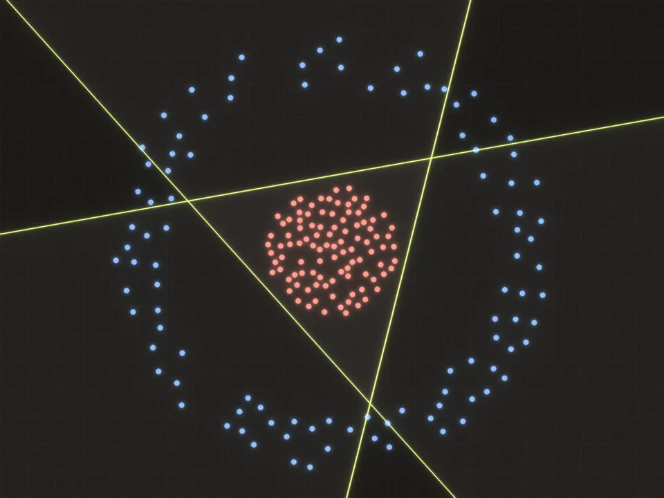 Each hidden neuron splits the plane with one line. Where all three agree is a triangle, and that is where the network says coral.
Two details from the walkthrough are worth putting into words. First, why tanh and ReLU look different. A tanh neuron's output goes from to across its line, smoothly, so the output neuron adds up soft steps and its boundary has rounded corners. A ReLU neuron's output is 0 on one side and a ramp on the other. The neurons' lines cut the plane into regions, and inside each region every ReLU is either off (0) or on (linear in and ), so the output's is a linear function there. Its boundary is therefore a straight segment inside each region, and the segments meet at corners where they cross from one region into the next. Second, why too few neurons fail. Each first-layer neuron contributes one line. A disc needs at least three lines around it; with two, the best the network can do is a stripe or a wedge, and no amount of training changes that. The universal approximation theorem from activations and initialization is the same statement from the other side: enough pieces can make any shape.
To recap: training moves every neuron's line a little on each step; the output layer combines the pieces into the boundary; and the number of hidden neurons limits how many pieces there are.
Now write the loop yourself, for three spiral arms. The setup provides the reference Linear and Tanh layers (the ones you wrote in backpropagation, plus the parameters() and grads() methods that list their arrays) and the data; you write the model, the evaluation, and the loop.
Write the full training loop and train a 2-64-3 tanh network to classify three interleaved spiral arms. The setup imports the reference Linear, Tanh, softmax_cross_entropy and make_spiral from mlref.nn.
MLP(n_in, n_hidden, n_out, rng): Linear, Tanh, Linear, withforward,backward,parameters()andgrads().evaluate(model, X, y): the mean cross-entropy loss and the accuracy, changing nothing.train(...): mini-batch SGD that records the training loss, validation loss and validation accuracy at step 0, everylog_everysteps and at the end, streams them withshow.line, and returns the history.
The last lines split the 300 points into 240 for training and 60 for validation, train for 3,000 steps and draw the decision regions. Once it passes, change the learning rate to 0.05 and to 20, or the hidden size to 4, and watch the curves.
This one trains a model in your browser, so a run can take a minute or more. The charts update as it goes, and Stop ends it early.
raise NotImplementedError, then press Run tests. Each check says what it expects.Reading the curves
A training run is an experiment, and its curves are the measurements. Most failures have a recognizable signature, so learning the signatures saves hours.
- The loss explodes, spikes, or becomes
nan. The learning rate is too high. Each step overshoots the bottom of the valley by more than it corrected, exactly the divergence you saw on a quadratic in gradient descent, where the step size had to stay below . Lower it by a factor of 3 to 10. (Gradient clipping, which caps the size of each step, is the standard safety net; module 7 needs it.) - The loss falls, but painfully slowly. The learning rate is too low, or the network started saturated (tanh units pinned at pass back almost no gradient) or with dead ReLUs. Check the size of the activations after the first forward pass, as in activations and initialization.
- The loss does not move at all. A bug: the update is not in place, the gradients are zero (all-zero initialization, or a backward pass that never ran), or the learning rate is zero. A gradient check and a step-0 loss near rule out most of these.
- The loss stalls on a plateau, then drops. Often normal. Networks can sit near a saddle point or a poor solution for a while before finding the way down. The widget below shows one, and what the neurons are doing during it.
- The loss stops falling at a level well above zero. If a larger learning rate and a longer run do not help, the network may be too small for the data: too few pieces, as step 6 above showed.
- The training loss keeps falling while the validation loss turns upward. Overfitting: the model has started to memorize the particular training examples, including their noise, instead of the pattern. Remedies: more data; a smaller model; stopping at the step where the validation loss was lowest (early stopping); or regularization, such as weight decay, which adds a small pull of every weight toward zero, or dropout, which randomly zeroes units during training.
The widget below is the same playground on a harder problem: two spiral arms wound around each other, 100 points each, and a 2-8-8-1 tanh network with 105 parameters. Its loss curve shows several of these signatures, depending on the settings. Keep an eye on the epoch and accuracy readouts, the loss curve under the network, and the eight layer-1 tiles.
The code below watches two of these signatures in the spiral classifier of the exercise, with three classes and 64 hidden units: it trains with three learning rates, then trains on only 45 of the 240 training examples for a long time.
Read the three learning rates first. At the loss drops to about 0.71 in the first few hundred steps and then barely moves. That is about what the best linear classifier (one whose three class regions are separated by straight lines) reaches on this data: a loss of about 0.72, with 55% accuracy. The network has found a rough, nearly linear split and has not yet found its way to the spiral. It is not broken, only slow: given ten times as many steps, it gets there. At the loss reaches about 0.06. At the loss ends far above where it started, in the tens or hundreds: each step overshoots, the logits blow up, and the model becomes confidently wrong.
Then the 45 examples. The training loss heads to zero, while the validation loss falls to its lowest point (about 0.78) around step 400 and then climbs past 2. The model is memorizing 45 points instead of learning a spiral. Early stopping would keep the weights from step 400.
Now read a pair of curves described in words.
You train a classifier and log both curves. The training loss falls steadily from 2.3 to 0.05 over 5,000 steps. The validation loss falls to 0.60 by step 1,500, then climbs to 1.40 by step 5,000, while the training loss keeps falling. What is happening, and what is a sensible response?
Choose one answer, then check.
To recap: an overshooting learning rate shows up in the training loss itself, a plateau is a flat stretch that ends, too few neurons is a floor that no setting lowers, and overfitting shows up only as a gap between training and validation.
Finally, put the whole checklist together, as you would for a colleague.
A client's team reports that their new classifier trained fine, because the training loss went down. What else would you ask to see or check before believing it, and what would each check reveal?
Saved in this browser as you type.
Everything here used plain gradient descent, where every parameter takes a step of times its own gradient. The next lesson derives the two optimizers that most real training uses instead, momentum and Adam, and the variant behind most large language models.