Vanishing and exploding gradients

The character RNN from the previous lesson learned to beat the bigram model, and its samples look like Shakespeare line by line. But little carries over from one line to the next. Is that the model's size, the training, or something deeper?

Something deeper. Backpropagation through time gets a loss's gradient to every earlier state, but on the way back the gradient is multiplied at every step by nearly the same factor. That is the repeated multiplication of powers, stability and explosion, and it makes the signal from far back either vanish or explode. This lesson follows one gradient back step by step, bounds its size in general, looks at what can be done about it, and ends with an experiment where a plain RNN fails a simple memory test. That failure is the reason for the LSTM of module 8.

#Follow one gradient back

Start with the smallest case, where every factor is a single number. In a scalar RNN, $h_t = \tanh(w\,h_{t-1} + u\,x_t)$, the rule from the previous lesson for the gradient arriving from step $t$ becomes

when $h_{t-1}$ affects the loss only through $h_t$ (it has no output loss of its own). In words: to go back one step, multiply by the recurrent weight $w$ and by the tanh slope $1 - h_t^2$ at the state being left. Call $w(1 - h_t^2)$ the factor of that hop.

The diagram below applies this rule over four steps. The RNN has $w = 0.8$, $u = 1$ and $h_0 = 0$ and reads the pulse $x = 1,\allowbreak 0,\allowbreak 0,\allowbreak 0$, the fading memory from the first lesson. The loss depends only on the last state, $L = h_4$. Boxes hold the states, amber arcs carry the gradient back one hop at a time with each hop's factor written on it, and a chart underneath collects the gradient after 0, 1, 2 and 3 hops on a log scale.

Now the general scalar case. Follow one loss term $\ell_t$ back $k$ steps. Each hop contributes its own factor, and the chain rule multiplies them:

The product runs over the $k$ states the gradient leaves on its way back, $h_t$ down to $h_{t-k+1}$. In the diagram, $t = 4$ and $k = 3$: the product is $w(1 - h_4^2) \cdot w(1 - h_3^2) \cdot w(1 - h_2^2) = 0.7200 \times 0.6659 \times 0.5636 = 0.2702$, the gradient at $h_1$. If the state hovers around some value $h$, every factor is about $\gamma = w(1 - h^2)$, and the product of $k$ of them is $\gamma^k$. Some numbers:

• $w = 0.9$ and states near $h = 0.5$: $\gamma = 0.9 \times (1 - 0.25) = 0.9 \times 0.75 = 0.675$. After 10 steps the gradient is $0.675^{10} \approx 0.0196$ of its size, after 20 steps $0.675^{20} \approx 0.000386$.
• $w = 1.5$ and states near $h = 0.6$: $\gamma = 1.5 \times (1 - 0.36) = 1.5 \times 0.64 = 0.96$. Slow decay, but decay: $0.96^{20} \approx 0.44$ and $0.96^{100} \approx 0.017$. A weight above 1 is not enough to keep the gradient alive, because the tanh slope is below 1.
• $w = 2$ with the state latched at $h = 0.9575$ (the first lesson's memory): $\gamma = 2 \times (1 - 0.9168) = 2 \times 0.0832 = 0.166$. A saturated state is a flat part of the tanh, and the gradient through it dies within a few steps, as step 8 of the diagram showed for $w = 1.8$. The very mechanism that held a memory in the forward pass blocks the learning signal in the backward pass.

The tanh slope is never more than 1, so each factor has size at most $|w|$. The gradient can only grow if $|w|(1 - h^2) > 1$, which needs $|w| > 1$ and states close enough to 0 that the tanh is steep there.

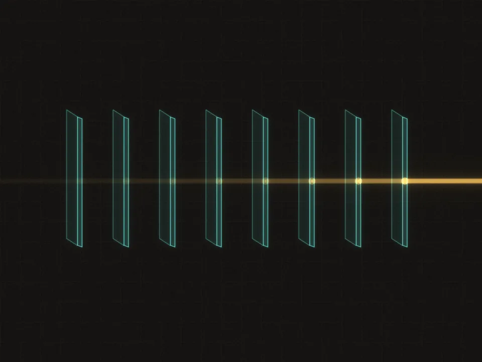Each step back is one more pane: the same fraction gets through every time, so the signal from far back fades geometrically.

Walk three hops yourself, through states that are not all alike. One hop grows the gradient and one shrinks it hard; see which and why.

When the states stay in one region, one number, $\gamma$, decides everything. Try it for a weight above 1.

#A product of Jacobians

A real RNN has many hidden units, so each factor is a matrix, not a number. The story is the same, with matrices. Between $\mathbf{h}_{t-k}$ and $\mathbf{h}_t$ lie $k$ recurrent steps, and each step is a function from the previous state to the next. Its Jacobian, the matrix of partial derivatives $\partial h_{s,i}/\partial h_{s-1,j}$, is

Here $\mathrm{diag}(\mathbf{v})$ is the diagonal matrix with the entries of $\mathbf{v}$ on its diagonal, so $\mathbf{J}_s$ is the recurrent matrix with row $i$ scaled by the tanh slope $1 - h_{s,i}^2$ of unit $i$. To see it, differentiate $h_{s,i} = \tanh\big(\sum_j (W_{hh})_{ij}h_{s-1,j} + \cdots\big)$ with respect to $h_{s-1,j}$: the chain rule gives the tanh slope $1 - h_{s,i}^2$ times the inner derivative $(W_{hh})_{ij}$. With one unit, $\mathbf{J}_s$ is the number $w(1 - h_s^2)$ from the previous section.

The chain rule is multiplication of Jacobians, so

with $\mathbf{J}_s^\top = \mathbf{W}_{hh}^\top\mathrm{diag}(1 - \mathbf{h}_s^2)$ (a diagonal matrix is its own transpose). The second formula is the gradient version. By the chain rule, $\partial\ell_t/\partial\mathbf{h}_{t-k}$ is the transpose of the Jacobian product times the gradient at $\mathbf{h}_t$, as in Jacobians and the chain rule, and transposing a product reverses its order: $(\mathbf{J}_t\cdots\mathbf{J}_{t-k+1})^\top = \mathbf{J}_{t-k+1}^\top\cdots\mathbf{J}_t^\top$. Read it from right to left: the gradient starts at $\mathbf{h}_t$ and is multiplied by one factor for every step it travels back, each factor being the previous lesson's rule, "through the tanh slopes, then through $\mathbf{W}_{hh}^\top$". After $k$ steps it has been multiplied by $k$ matrices, each built from the same $\mathbf{W}_{hh}$.

A bound from singular values

With matrices we cannot just multiply numbers, but we can bound how much each factor stretches. In symmetric matrices and the SVD the largest singular value $\sigma_1$ was the gain of a matrix: $|\mathbf{A}\mathbf{v}| \le \sigma_1(\mathbf{A})|\mathbf{v}|$ for every $\mathbf{v}$. Each backward factor does two things:

1. It multiplies the entries of the gradient by the slopes, each between 0 and 1, which cannot make it longer.
2. It multiplies by $\mathbf{W}_{hh}^\top$, which has the same singular values as $\mathbf{W}_{hh}$ and so stretches by at most $\sigma_1(\mathbf{W}_{hh})$.

So each step back can stretch the gradient by at most $\sigma_1(\mathbf{W}_{hh})$, and after $k$ steps

If $\sigma_1(\mathbf{W}_{hh}) < 1$, the gradient from $k$ steps back is guaranteed to shrink at least geometrically: vanishing is certain. If $\sigma_1 > 1$ the bound allows growth but does not force it, because the tanh slopes may pull every factor below 1, as they did for $w = 1.8$ in the diagram.

The eigenvalue view

The singular-value bound holds for any states. When the states settle into a steady pattern, we can say more. The factors are then nearly the same matrix $\mathbf{J}$ every step, and a product of $k$ copies behaves like $\mathbf{J}^k$. The eigenvalues of powers, stability and explosion take over: the gradient scales like $\rho(\mathbf{J})^k$, where $\rho(\mathbf{J}) = \max_i |\lambda_i|$ is the spectral radius, the size of the largest eigenvalue ($\mathbf{J}^\top$ has the same eigenvalues as $\mathbf{J}$).

Now think about what holding a memory requires. A state that stores something robustly sits at a fixed point that pulls nearby states back toward it, so that small disturbances die out instead of wiping the memory. Pulling nearby states back means the Jacobian shrinks small differences, so $\rho(\mathbf{J}) < 1$, and the gradient, which travels back through the same Jacobians, shrinks too. Storing information robustly and passing a learning signal back through it pull in opposite directions. The scalar latch above is the one-unit version: its factor $0.166$ is also how much a small disturbance of the stored state shrinks at each step, which is what makes the memory robust and the gradient vanish.

Watching it happen

The instrument below runs the matrix version on a random RNN with 8 tanh units. Its recurrent matrix is $\mathbf{W}_{hh} = \rho\,\mathbf{Q}$, where $\mathbf{Q}$ is a fixed random orthogonal matrix (every singular value 1), so $\rho$ is both the spectral radius and the largest singular value of $\mathbf{W}_{hh}$. The chart plots $\|\partial\mathbf{h}_T/\partial\mathbf{h}_{T-k}\|$ against the number of steps back $k$, from 0 to 80: the spectral norm of the whole product of $k$ Jacobians, written with double bars as in symmetric matrices and the SVD, the most it can stretch any gradient. The vertical axis is a log scale, so geometric decay or growth is a straight line. A toggle includes the tanh slopes or leaves them out.

The same experiment in code, with a 64-unit RNN driven by random inputs. G is a random matrix with spectral radius close to 1 (and largest singular value close to 2), and W_hh is G times a scale. The code walks a gradient of length 1 back from the last state with the previous lesson's rule and records its length after every step.

At scales 0.5 and 1 the gradient from 80 steps back is smaller than $10^{-13}$ of where it started. At scale 4 it is larger than $10^{12}$. Only in a narrow band around scale 2 does it stay within a few powers of ten, and nothing in training keeps $\mathbf{W}_{hh}$ inside that band. Notice also which way the singular-value bound works. At scale 1 the largest singular value is about 2, so the bound allows growth by up to $2^{80} \approx 10^{24}$, yet the gradient vanished: the tanh slopes and the directions of the matrices did the rest. A bound below 1 guarantees vanishing; a bound above 1 guarantees nothing.

To recap: going back $k$ steps multiplies the gradient by $k$ factors built from the same $\mathbf{W}_{hh}$ and the tanh slopes; their size is at most $\sigma_1(\mathbf{W}_{hh})^k$; saturated states make the factors smaller still; and in practice the result is geometric decay or growth.

#What vanishing does to learning

Why does a tiny gradient from far back matter, if the gradient from nearby steps is fine? Because every weight update adds them together. Every entry of $\partial L/\partial\mathbf{W}_{hh} = \sum_t \boldsymbol{\delta}_t\mathbf{h}_{t-1}^\top$ is a sum of contributions, and each contribution links a loss at some step to a state some number of steps $k$ earlier, scaled by roughly $\gamma^k$.

With $\gamma = 0.7$, a link one step long counts $0.7$, a link five steps long counts $0.7^5 \approx 0.17$, and a link 20 steps long counts $0.7^{20} \approx 0.0008$. The long-range contributions are in the sum, but they are drowned out by the short-range ones. Gradient descent follows the sum, so it learns the short-range patterns and barely sees the long-range ones.

#What can be done

The two problems are not symmetric, and neither are their remedies.

Exploding gradients: clip them. This is the clipping of the previous lesson. When the product of factors blows up, clipping by norm caps the length of the whole gradient and keeps its direction, so one bad batch cannot throw the weights far away. It treats the symptom, a step that is too long, and that is enough in practice.

Vanishing gradients: no simple fix. Clipping cannot help, and neither can scaling the gradient up, because the problem is relative: the long-range contributions are tiny compared with the short-range ones in the same sum, and scaling multiplies both. Optimizers such as Adam, which divide each weight's step by the typical size of its gradient, help when a gradient is small but consistent; they cannot pull a faint long-range signal out from under larger short-range contributions to the same weights. Careful initialization (a recurrent matrix close to the identity, or an orthogonal one, whose singular values are all 1) helps at the start of training, but nothing keeps the matrix there. The fix that worked was a change of architecture: give the network a memory path along which the per-step factor is a number the network controls and can hold near 1. That is the cell state of the LSTM, the subject of the next module.

Truncated backpropagation through time. A different, practical limit also cuts long-range learning. A long text cannot be unrolled all at once: the forward pass stores every state, so memory grows with every step. The usual compromise cuts the text into consecutive chunks of $T$ steps and treats the two directions differently:

• The forward pass carries the state across chunk boundaries: the last state of one chunk becomes $\mathbf{h}_0$ of the next, so the model can still carry information forward indefinitely.
• The backward pass stops at the boundary: the carried-in $\mathbf{h}_0$ is treated as a constant, so no gradient crosses into the previous chunk.

The model can use information from further back than $T$ steps, but it gets no training signal telling it to keep such information. The training in the previous lesson was simpler still: every window was cut from a random place and started from a zero state, so the model never saw more than 32 characters of context while it trained.

Check that you can tell apart what truncation keeps and what it cuts.

#Where the plain RNN breaks: delayed recall

Everything so far says the long-range signal is weak. A clean experiment shows how weak, with a task that needs memory and nothing else. The delayed-recall task uses 9 tokens: four symbols (ids 0 to 3), four noise tokens (ids 4 to 7) and a cue (id 8). Each sequence is

where $s$ is a random symbol, the $n_i$ are $d$ random noise tokens, and $d$ is the delay. For example, with $d = 3$ one sequence might be 2, 5, 7, 4, 8, 2: the symbol 2, three noise tokens, the cue, and the symbol again.

The model is trained exactly like the language model: predict the next token at every position, with teacher forcing and the average cross-entropy. Most targets are noise tokens, which nothing can predict better than a one-in-four guess. The one that matters is the last: the token after the cue is $s$, which was read $d + 1$ steps earlier. Guessing gives 25% accuracy at that position; remembering gives 100%.

This is the previous sections in miniature. The gradient that could teach the network to store $s$ comes from a single position and has to travel back $d + 1$ steps, while the noise positions contribute larger, short-range gradients to the same weights.

In our runs the RNN solves delays 2, 4 and 8 completely. At 16 the outcome depends on the run: with some random seeds it learns the task, with others it gets partway or stays at chance. At 24 and 32 it stays at chance, 25%: after 800 training steps its answers show no trace of $s$. Training longer moves the boundary out only slowly, because each extra step of delay multiplies the useful signal by another factor below 1. Module 8 runs a version of this experiment, set up as a classifier that answers once at the end, with an RNN and an LSTM side by side, and the LSTM keeps learning at delays where the RNN usually fails.

To finish the module, explain the whole chain of reasoning in your own words, from the product of factors to the fix.