
Lesson 1 of 5
Sequences and state
A recurrent network reads a sequence one element at a time and carries a hidden state from each step to the next, using the same weights at every step. Unrolled through time, it is a deep network whose layers all share one set of weights.
Explain why a fixed-size network cannot read text of any length, and what a hidden state adds.
Run a recurrent network forward by hand, for a scalar state and for a vector state.
Explain why a matrix times a one-hot vector is a table lookup, and what an embedding table is.
Count the parameters of a recurrent network and explain why the count does not depend on the sequence length.
Implement the forward pass of a character RNN over a batch of sequences, keeping the cache that backpropagation needs.

Here is the first line of speech in the Shakespeare text you will train on in this module:
Before we proceed any further, hear me speak.
Suppose you want a network that reads it one character at a time and, after every character, guesses the next one. After "procee" it should be almost sure of "d". After "hear me " it has many reasonable options. And the right guess depends on more than the current character: in "hello" the first "l" is followed by another "l", the second by "o". Both times the network has just read an "l", so to tell the two apart it has to remember what came before.
Every network in module 6 takes a vector of one fixed size and returns a vector of one fixed size. A line of text has no fixed size, and a whole play certainly does not. This lesson builds the network that handles sequences: the recurrent neural network, or RNN. It reads one element at a time and carries a small vector, its state, from each step to the next. By the end you will have written its forward pass for batches of text, which the rest of this module turns into a trained language model.
Text has no fixed size
Why can we not just use the networks we already have? Two obvious ways to feed text to a fixed-size network both fail, and the ways they fail show what we need.
Feed the whole text at once. Turn each character into a vector (the section on characters as vectors makes this precise) and concatenate them. A 1,000-character passage over a 60-character alphabet becomes a vector with entries. Three problems follow. Texts have different lengths, so everything must be padded to the longest one. Every position gets its own weights, so what the network learns about "the" at position 5 tells it nothing about "the" at position 500: it has to learn every pattern again at every position. And the number of weights grows with the length of the text.
Feed a fixed window. Keep only the last characters, say , and predict the next one from those. The window slides along the text, so the same weights serve every position, and any length is fine. This is the idea behind classic n-gram language models; the bigram model in the next lesson is the case . But anything older than characters is invisible. Whether an open quotation still needs closing, or which character in the play is speaking, can depend on something 50 or 500 characters back.
What we want is a model that reads any length, applies the same rule at every position, and can remember what matters from far back.
The idea: carry a state. You already know a machine like that. To add up a list of numbers of any length, keep one number , start it at 0, and at every step do . One rule, repeated; a state of fixed size (one number); any length.
Here is a more interesting one: a counter of open parentheses that adds 1 for "(", subtracts 1 for ")" and ignores everything else. Feed it the 9 characters of f(a, g(b) one at a time. After each character the counter reads
It ends at 1, so one closing parenthesis is still owed, however long ago the first one opened. The counter never looks back at the text. Everything it needs about the past is in one number, which it updates with the same rule at every character.
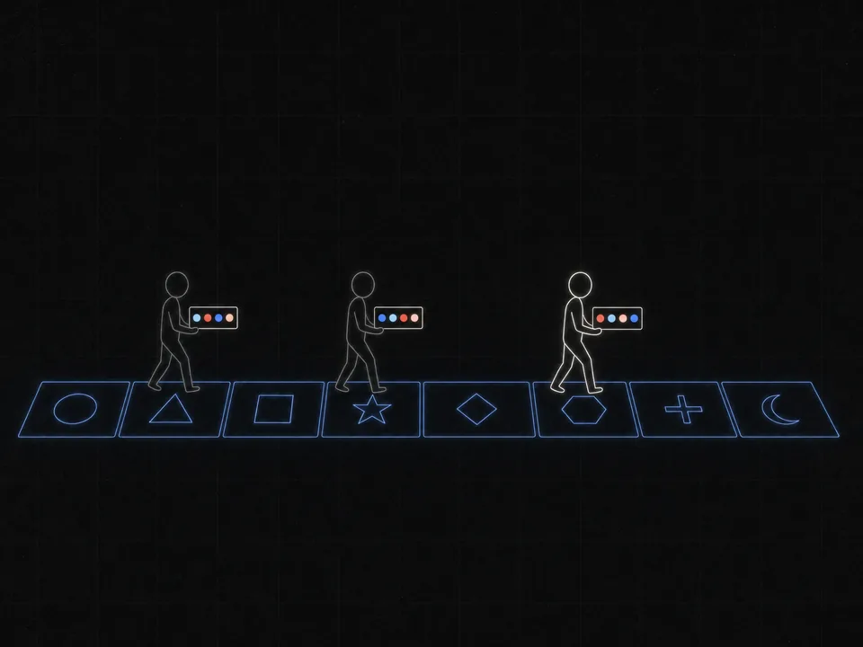 Reading with a state: one step per element, and a summary of fixed size, updated at every step and carried to the next.
A recurrent network is this idea with two changes: the state is a vector of numbers instead of one counter, and the update rule is learned from data instead of written by hand.
The recurrent step
With the idea in place, we need the actual rule . The RNN's rule is a dense layer, the kind from module 6, applied to the previous state and the current input together:
Every symbol, in words:
- counts the steps, one per element of the sequence, and is the sequence length.
- is the input at step , a column vector with entries.
- is the hidden state after reading , a vector with entries; is the hidden size. The starting state is usually all zeros.
- () says how the previous state feeds the new one. These are the recurrent weights. The subscript reads "from h to h".
- (, "from x to h") says how the input feeds the new state, and is a bias with entries.
- acts on each entry separately and squashes it into , as in derivatives as zoom.
- is the output at step , with entries, read from the state by () and the bias . For a language model these are scores (logits) for the next character, which the next lesson turns into probabilities. Many sources call this output ; we save for the target, the character that actually comes next.
We will also name the sum inside the tanh. The pre-activation is , so that .
Why call it a dense layer? The two products can be written as one matrix acting on the previous state and the input stacked into one tall vector:
On the right, the matrix is and placed side by side, , and the vector is stacked on top of , with entries. Multiplying them row by row gives the first columns times plus the last columns times , which is the left side. So each step is exactly the neuron layer of module 6, whose input happens to include its own previous output. The LSTM in module 8 stacks its inputs the same way.
A scalar RNN
The smallest case lets us watch the state by hand. With every matrix is a single number. Take , , and , and feed a single pulse: . Each row of the table does one step: first the pre-activation from the previous row's state, then .
| 1 | 1 | 0.7616 | |
| 2 | 0 | 0.5436 | |
| 3 | 0 | 0.4094 | |
| 4 | 0 | 0.3163 | |
| 5 | 0 | 0.2478 |
The state remembers the pulse, but it fades. Each step multiplies it by , and then tanh shrinks it a little more. The ratios of consecutive states show both effects: , then , and . They climb toward because a small state sits where tanh is nearly a straight line, , so tanh stops shrinking it.
Now make the recurrent weight larger, , and feed the same pulse. The states are , then , then , then and , settling at . That value is where the rule stops changing the state: . It is the positive solution of . The state no longer fades.
But feed a pulse of instead of and the state starts lower, , then , and it keeps climbing to the same . Feed and it settles at . This network remembers the sign of the pulse and forgets its size.
Neither is a good memory. With the memory fades; with it latches onto a single bit. Which behavior you get depends on the recurrent weight, applied again at every step. That repeated multiplication is the thread of this whole module, and it is the reason for module 8, the LSTM.
A vector RNN
The same step with vectors is a matrix-vector product, a vector addition and a tanh on each entry. With two hidden units and one input, take
Build the pre-activation piece by piece. First the recurrent term. Row of says how much unit listens to each unit's previous value (the row view from matrices as transformations), so entry is row dotted with :
Then the input term. The input is a single number, so is the column scaled by 2:
Add the two terms and the bias entry by entry, then apply tanh to each entry:
The stacked form from the start of this section gives the same sum in one product. Place and side by side and stack on top of :
which is the recurrent term plus the input term, . Adding gives the same .
To recap: one step is (1) the recurrent term , (2) the input term , (3) add them and the bias, (4) tanh each entry. The next step starts again from the you just computed, with the same three weights.
Now run the step yourself. The first part feeds two inputs through a scalar RNN, so you see how the state carries the first input into the second step; the last part is one vector step like the one above.
Work these by hand with , keeping four decimals in every intermediate value.
- A scalar RNN has , and . Starting from , feed and then . Find and .
- Redo part 1 with instead of . Which of and change, and what does that say about what carries?
- A two-unit RNN with one input has , and . Find for and .
To check your work, enter four numbers as a column: and from part 1, then the two entries of from part 3, unit 1 first.
Work it on real paper: writing each step is the point. Then check your final answer here and compare your working with the walk-through.
One entry per box, top to bottom. 0.25, -2, 3/4 and sqrt(2) all work. Enter moves to the next empty box and checks once all are filled.
For more practice, here is an unlimited set of steps with fresh numbers: two scalar steps or one vector step each time.
A two-unit RNN computes with applied to each entry. Use , , , the previous state and the input . Find to 3 decimal places.
One entry per box, top to bottom. 0.25, -2, 3/4 and sqrt(2) all work. Enter moves to the next empty box and checks once all are filled.
In code, batches are rows
Everything above uses column vectors, one sequence at a time. Code runs sequences at once and stores their states as the rows of a array, as in shapes, transposes and batches. To see what the code must hold, transpose the step for one sequence, turning every column into a row. Three facts do it. The tanh acts on each entry by itself, so it gives the same numbers whether they sit in a column or a row. Transposing a sum transposes each term. And transposing a product reverses its order, . So, writing the input term first as code does,
The states and inputs are now rows, and the matrices are transposed. So in code Wxh holds with shape (m, n), Whh holds with shape (n, n), and Why has shape (n, K). One step for the whole batch is
h = np.tanh(x @ Wxh + h @ Whh + bh) # x: (B, m), h: (B, n), bh: (n,) added to every rowCheck it on the vector example. There Whh is and the state is the row [1, -1]. Then h @ Whh is , the same two numbers as . Likewise Wxh is the row [0.5, -1], and x @ Wxh with x = [[2]] gives [[1, -2]]. The numbers are the same; only the layout is transposed. The course's reference code in mlref/rnn.py follows this convention, and the lesson formulas keep column vectors.
Unrolling: one network, many layers
We have a rule for one step. What does the whole computation over a sequence look like? Write out the first three steps:
Now substitute. Replace in the third line by the right side of the second line:
then replace by the right side of the first line:
Read from the inside out, that is three dense layers applied one after another: a three-layer feed-forward network. Drawing the steps side by side, left to right, is called unrolling the network in time.
The instrument below unrolls a small RNN over the word "hello". It answers two questions: what happens at each step, and which weights each step uses. Each column is one time step. At the bottom of a column is the one-hot input, one row per character of the vocabulary with the row of the character read lit up; above it is the hidden state, 4 units shown as colored cells (coral above 0, blue below 0). Blue arrows carry the input into the state through , lime arrows carry the previous state across through . The weights are fixed random numbers, not trained ones, so the states mean nothing yet; what matters is how they are computed.
The unrolled network is unusual in two ways. First, every layer uses the same weights: , and appear at every step. These are called tied or shared weights. Second, a fresh input enters at every layer, and an output can leave at every layer. A sequence of length becomes a network layers deep.
Sharing weights across time is the same move a convolutional network makes across space, where one small filter slides over every position of an image (you meet it in module 9). It buys three things:
- Any length. The same step runs as many times as there are characters.
- Patterns transfer across positions. What the network learns about "the" at step 5 is used at step 500, because it is the same weights.
- A fixed number of parameters. Reading ten characters or ten thousand uses the same matrices.
It also costs something. A long sequence makes a very deep network, and every layer multiplies by the same . You saw in powers, stability and explosion what repeated multiplication by one matrix does, and the last lesson of this module, vanishing and exploding gradients, shows what it does to training.
One more property falls out of the unrolled picture: depends only on . In the widget, the columns to the right of the step shown stay dashed: the state at step has not seen the future, which is exactly what a model that predicts the next character needs.
Before moving on, check that the unrolled picture is clear: what it multiplies, what it shares, and what each state can see.
An RNN with hidden size 128 is unrolled over a sequence of 50 characters. Which statement is true?
Choose one answer, then check.
Characters as vectors
So far the input has been any vector of numbers. Text is characters, so we need a way to turn a character into a vector, and the way we choose turns out to make the input term almost free to compute.
Each character gets an id: its position in a sorted list of all the characters that occur, the vocabulary. With a vocabulary of characters, the one-hot vector of character is : entries, all 0 except a 1 in position . For a vocabulary {a, b, c}, the character b is . (Math counts positions from 1 and Python from 0, so in code the same b has id 1 and its one-hot vector is np.eye(3)[1].)
Now look at what the input term does with a one-hot vector. The column view of a matrix times a vector (matrices as transformations) says is times column 1 plus times column 2, and so on. With , every coefficient is 0 except the -th, so
For example, take and feed b, which is . The column view gives
the second column. No multiplications are needed: a matrix times a one-hot vector is a table lookup. Each character owns one column of , and that column is what the character adds to the pre-activation every time it is read. In code, where Wxh has one row per character, the lookup for a whole batch of ids is Wxh[ids], which equals one_hot(ids) @ Wxh without building the one-hot arrays.
Try one full step where the input is a one-hot character: the input term becomes a lookup, and the rest is the vector step you already know.
A two-unit RNN reads characters from the vocabulary {a, b, c} as one-hot vectors. Its weights are , and . The previous state is , and the network now reads c. Find to 3 decimal places, and enter it as a column, unit 1 first.
One entry per box, top to bottom. 0.25, -2, 3/4 and sqrt(2) all work. Enter moves to the next empty box and checks once all are filled.
Embeddings. Look at what the RNN has already learned in : every character owns a column of numbers, trained by gradient descent, that stands for that character inside the network. That column is a learned vector for the character.
Larger models make this explicit with a separate embedding table , a matrix with one row per token: row is a learned vector of numbers that stands for token . Looking a token up is the same one-hot trick from the other side, row of , and the network then works with those -number vectors instead of -entry one-hot vectors. The table is trained like every other weight. Tokens that behave alike tend to end up with vectors that point in similar directions, which is why the cosine similarity of length and similarity is the usual way to compare them.
What does an embedding change for the RNN above? Follow one character through it in three moves:
- Look up the embedding: , row of written as a column of numbers.
- Multiply by the input weights, which now take numbers in, so is : the input term is .
- Regroup the product: , which is column of the matrix .
So it is still one lookup, into a matrix built as the product of two thin ones, and therefore of rank at most (inverses, systems and rank). It stores numbers instead of , which is fewer whenever . For characters, and : numbers instead of . The table can also be shared with other parts of the model.
Run the example below. It builds the one-hot vectors for "hello world", checks that the product is a lookup, and runs a small RNN with random weights over the text.
The two l's add the same row of Wxh (the same column of in the math) but produce different states, because the previous state differs. The state after "hel" carries "he" with it; the state after "hell" carries "hel". This is the effect you saw at steps 3 and 4 of the instrument, now in code.
Counting parameters
One of the promises of weight sharing was a parameter count that does not grow with the text. Here is the count, piece by piece: has entries, has , has , has and has . Group the first three (they all have rows) and the last two (they all have rows):
For a character model over our Shakespeare text, the inputs and the outputs are both one-hot over characters, so . With hidden size :
More than half of that is , with entries. None of it depends on .
Compare the fixed-window alternative. A network that reads the last 100 characters as one-hot vectors has inputs, and a first layer of 128 units already needs weights, 24 times the entire RNN, while still seeing nothing older than 100 characters.
The work per character is also fixed. Each step costs multiply-adds for (the input term is a lookup) and for the output: for this model, whether it has read 10 characters or 10,000. A transformer in module 9 works differently: each new token looks back at every earlier one, so its cost per token grows with the context.
Count one yourself, for a bigger vocabulary and a bigger state.
A character RNN reads one-hot characters from a vocabulary of 80, has hidden size 256, and outputs logits over the same 80 characters. How many parameters does it have, biases included? Enter the whole number, without commas.
Type a number: 0.25, -2, 3/4 and sqrt(2) all work. Enter checks.
Write the forward pass
Recap before you code: one step is ; a one-hot input makes a lookup; code stores the transposed matrices and keeps a batch of sequences as rows; the output layer reads logits from every state.
Here is everything the forward pass has to do for a batch, in the code layout:
- Look up the input rows for every step at once,
Wxh[X]. - Loop over time, applying the recurrent step. This loop is the one part that cannot run in parallel, because each state needs the one before it.
- Compute the logits for every step with one matrix product.
- Keep a cache: every hidden state it produced, the inputs and the starting state. Backpropagation in backpropagation through time needs all of them, just as the layers of module 6 kept their inputs for the backward pass.
Write the forward pass of a character RNN for a batch, in the code layout (batches are rows, and Wxh has shape (V, H)).
one_hot(ids, V): one-hot vectors for an array of ids of any shape.rnn_step(x_onehot, h_prev, params): one step for a batch,tanh(x @ Wxh + h @ Whh + bh).rnn_forward(params, X, h0=None): run a batch of id sequences of shape(B, T)and return the logits(B, T, V), a cache of everything backpropagation will need, and the last state. Use the lookupWxh[X]rather than one-hot products, so the only work inside the time loop is the recurrent product.
The tests compare your results with the course's reference implementation in mlref/rnn.py.
raise NotImplementedError, then press Run tests. Each check says what it expects.To finish, put the whole lesson in your own words, as you would for a colleague who knows ordinary networks well.
A colleague knows multilayer perceptrons well but has never used a recurrent network. Explain how an RNN reads text of any length, what "unrolling" means, and what sharing the weights across time buys and costs.
Saved in this browser as you type.