
Lesson 4 of 4
Length and similarity
How long is a vector, how far apart are two of them, and how closely do their directions agree? Cosine similarity is the dot product with length divided out, and it is how embedding search compares meaning.
Compute the L2 and L1 lengths of a vector in any number of dimensions, and normalize a vector to length 1.
Choose between distance and angle for a comparison, and compute cosine similarity by hand and in code.
Prove the Cauchy-Schwarz inequality and explain why it keeps cosine similarity between -1 and 1.
Build nearest-neighbor search and word analogies over a small embedding table.

Suppose you are building search for a help center. As a first attempt, you describe each article by how many times three words appear in it: password, reset and invoice. A user types "reset password", which becomes the query vector .
Article is a short note on resetting your password: . Article is a long billing FAQ that mentions passwords along the way: . Score both with the dot product:
The billing FAQ wins, mostly because it is long. Worse, if the password note is accidentally saved with its text pasted in twice, its counts double to and its score doubles to , although it has not become any more relevant. The dot product mixes two things: how closely two vectors point the same way, and how long they are. For search we usually want only the first.
This lesson pulls the two apart. First length, then direction, then the inequality that makes "angle" meaningful in any number of dimensions, and finally a small embedding search you build yourself.
How long is a vector
Before we can divide length out of a comparison, we need a way to measure it. In the plane, a vector and its two entries form a right triangle: the entries are the two short sides (the legs), and the arrow is the longest side (the hypotenuse). Pythagoras gives its length.
The figure shows exactly that triangle. The vector is drawn from the origin, its dashed legs show the two entries, and the second formula under the sentence computes the length by Pythagoras with the current numbers.
For that is . In three dimensions, Pythagoras is applied twice: has length . The picture below shows why twice is enough.
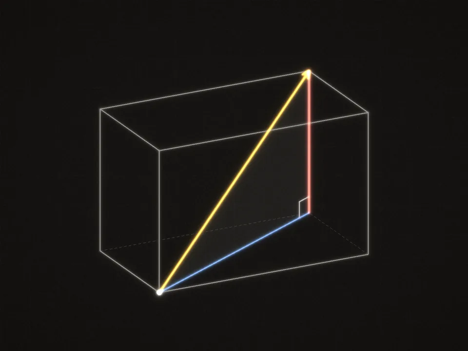 Pythagoras twice. The floor diagonal and a vertical edge meet at a right angle, so together with the arrow through the box they form a right triangle.
Go slower: Pythagoras twice, for three dimensions
Take . Its shadow on the floor (the plane where the third entry is 0) is .
Step 1, the floor. The shadow lies in a plane, so ordinary Pythagoras gives its length: .
Step 2, straight up. From the tip of the shadow, go straight up by to reach the tip of . Straight up is perpendicular to the floor, so the shadow, the vertical segment and form a right triangle with as its hypotenuse. Pythagoras once more: Squaring a square root gives back what was under it:
Step 3, the pattern. For : the shadow has length , and then . Each extra dimension adds one more perpendicular leg and one more squared entry under the root. Beyond three dimensions there is nothing to draw, so we take the pattern as the definition: every axis is perpendicular to all the others, and each one adds its squared entry.
The length (also called the Euclidean length, the magnitude or the L2 norm) of a vector with entries is
The second form is the one to remember: the dot product of a vector with itself is the sum of its squared entries. Many books and papers write the length with double bars, or , to keep it apart from the absolute value of a number. It means the same thing as our .
Two properties follow from the formula. First, the length is zero only for the zero vector, because a sum of squares is zero only when every entry is zero. Second, scaling a vector by scales its length by , the size of without its sign. One move per line:
- By the definition, .
- Square each product, : this is .
- Factor out : .
- The square root of a product is the product of the square roots: .
- , and the second root is : so .
The step matters: lengths are never negative, so is twice as long as , not times. Check: has length .
Unit vectors
Often only the direction of a vector matters. A unit vector has length 1, so it carries a direction and nothing else. Dividing any nonzero vector by its length gives the unit vector pointing the same way, a step called normalizing:
The hat means "the unit vector in the direction of". Its length is 1 by the scaling rule with , which is positive: . For , , and indeed .
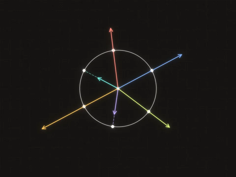 Normalizing moves each tip along its own arrow onto the circle of radius 1. The direction stays; the length becomes 1.
In the plane, every unit vector ends on the circle of radius 1 around the origin, the unit circle. Normalizing slides a tip along its own arrow, in or out, until it reaches that circle.
Normalizing is two steps: find the length, then divide every entry by it. The next vector has three entries and a zero among them.
Normalize : find the unit vector that points the same way. Enter its three entries top to bottom, as decimals or fractions.
One entry per box, top to bottom. 0.25, -2, 3/4 and sqrt(2) all work. Enter moves to the next empty box and checks once all are filled.
Another way to measure size
The L2 length measures the straight line from the origin to the tip. The L1 length measures the walk if you may only move along the axes, like a taxi on a grid of streets:
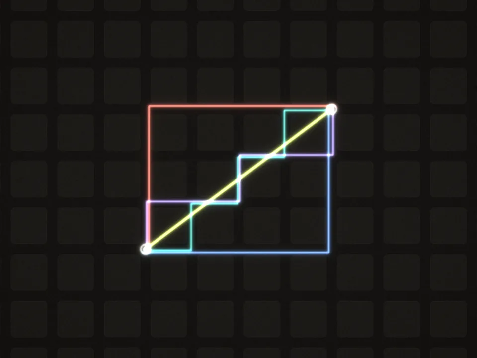 The straight line is the L2 length. Every route along the streets without backtracking has the same, longer length: the L1 length.
For the L1 length is , while the L2 length is . The walk along the grid is never shorter than the straight line, so always. To see why in the plane, square the L1 length: , which is the squared L2 length plus a term that is never negative. For : . (Other sources write .) In the plane, the vectors with L2 length 1 form the unit circle; those with L1 length 1 form a diamond with corners at and .
You will mostly meet the L1 length as a penalty during training. Adding to a model's loss, where (the Greek letter lambda) is a small positive number that sets the strength, favors solutions in which many weights are exactly zero. Adding instead (the squared L2 length, the usual choice in neural networks and closely related to what optimizers call weight decay) shrinks every weight but rarely makes any of them exactly zero.
The difference is in the pull, meaning the slope of the penalty, which is what gradient descent follows (module 5). The L1 penalty pulls a weight toward zero with the same strength however small the weight already is. The squared penalty pulls with strength , which fades to nothing as approaches zero. With and a weight of , the L1 pull is still , while the squared penalty pulls with , fifty times weaker. At the best weights the penalty's pull must balance the pull of the rest of the loss. Under L1, whenever the rest of the loss pulls a weight away from zero with strength less than , the penalty wins and the weight stays at exactly zero. Under the squared penalty the pull near zero is tiny, so any pull at all from the rest of the loss moves the weight to a small nonzero value.
To recap the section: the length is Pythagoras in any number of dimensions, scaling by multiplies it by , and dividing by it gives a unit vector. The L1 length adds the sizes of the entries instead, and it is never smaller.
Distance or direction
With length in hand, we can compare two vectors in two different ways, and they do not always agree.
The distance between and is the length of their difference, : the length of the arrow from the tip of to the tip of that you met in Arrows and lists.
Take , and :
By distance, is nearer to than is. Yet points exactly the same way as , while is perpendicular to it. Distance mixes direction and length. Sometimes that is right: two apartments with similar area, bedrooms and age should count as close, and their sizes matter. Sometimes it is wrong: a query and a long document about the same thing should count as similar however long the document is.
For direction alone, use the angle. The dot product lesson showed that , where is the angle between the arrows. Divide both sides by (for nonzero vectors):
This number is the cosine similarity of and . Linearity of the dot product shows what it really is. Dividing by is multiplying by and by . Linearity lets the first factor scale and the second scale , since and the same holds for the second vector:
Cosine similarity is the dot product of the normalized vectors. Normalize both, then dot. Stretching either vector changes nothing, because the stretch cancels in the division. The value is when the vectors point the same way, when they are perpendicular and when they point in opposite directions. In the example, with and , so
The figure from the dot product lesson shows the difference between length and angle directly. It draws (blue) and (coral) from the origin, the lime shadow of on the line of , and the amber arc for the angle, with readouts for , the angle, and the shadow. The question here: when you stretch one arrow, what changes and what does not?
Back to the help center. With cosine similarity, the password note scores
a perfect match in direction. The billing FAQ has , so it scores . The ranking now follows the topic, and pasting the note twice changes nothing: points the same way as , so its cosine with is still 1.
Distance and angle are not unrelated. Expanding with the dot product gives , as in the dot product lesson's derivation. When both vectors have length 1, the lengths drop out and only the angle is left.
Go slower: Distance between unit vectors
Let and have length 1, so and , and let be the angle between them, so .
Step 1. Squared length is the dot product with itself: Step 2. Expand with linearity, as you would multiply out : Step 3. Order does not matter, so and the middle terms combine: Step 4. Substitute the three known values:
The right side goes down exactly when goes up. So among unit vectors, the nearest one by distance is always the most similar one by cosine, and sorting by either gives the same order. Two unit vectors apart have , so and their distance is .
So the choice is not really between two unrelated measures. It is whether length should count. If it should not, normalize, and then distance and cosine agree.
To recap: distance counts both length and direction. Cosine similarity counts direction only. For unit vectors the two agree, because .
The next exercise works every measure from this lesson so far on one pair of 3D vectors, and checks the distance two ways.
Let and . By hand:
- The L2 length and the L1 length .
- The unit vector .
- The cosine similarity of and , as a fraction and as a decimal.
- The distance , two ways: directly, and from .
Enter four numbers in the check box, top to bottom: , , the cosine similarity and the distance, the last two to 3 decimal places.
Work it on real paper: writing each step is the point. Then check your final answer here and compare your working with the walk-through.
One entry per box, top to bottom. 0.25, -2, 3/4 and sqrt(2) all work. Enter moves to the next empty box and checks once all are filled.
Now a cosine on its own, in four dimensions. Compute the three ingredients separately, then divide.
Find the cosine similarity of and . Enter it as a decimal to 3 decimal places.
Type a number: 0.25, -2, 3/4 and sqrt(2) all work. Enter checks.
Distance and cosine can disagree when lengths differ a lot. The next question has one query and two documents, one of them three times as long as the query.
A query vector is . Document A has vector and document B has vector . Which document does each method rank closer to the query?
Choose one answer, then check.
Why cosine stays between −1 and 1
In the plane, is the cosine of an angle you can see, so it lies between and like every cosine. But for two 4,096-entry embeddings there is no angle to see. There, the formula is how we define the angle, and that only works if the ratio can never leave the range from to . The guarantee is the Cauchy-Schwarz inequality:
with equality exactly when one vector is a multiple of the other. Divide both sides by (for nonzero vectors) and it says . For the pair and : and , and indeed .
The picture behind it is the shadow from the dot product lesson. The shadow of on the line through has length (ignoring its sign), and a shadow is never longer than the arrow that casts it: the shadow and the drop form a right triangle with as the hypotenuse. "Shadow at most ", multiplied through by , is Cauchy-Schwarz.
Go slower: Proof of Cauchy-Schwarz from the projection
If , both sides are and there is nothing to prove. Otherwise, split into its projection on and a leftover, exactly as in the dot product lesson:
Step 1, the leftover is perpendicular. Dot with and use linearity: Substitute . The on top cancels the one underneath: Since is a multiple of , linearity gives too.
Step 2, Pythagoras. Since , the squared length of is Expand with linearity, as you would multiply out : Order does not matter, so and the two middle terms combine: The middle term is by step 1, and each self dot product is a squared length: A squared length is never negative, so dropping can only make the right side smaller:
Step 3, the length of the shadow. By the scaling rule, . Substitute : One factor of cancels, and :
Step 4, combine. Steps 2 and 3 give . Multiply both sides by , which is positive: . Both sides are nonnegative, so taking square roots keeps the inequality: .
When is it an equality? Steps 3 and 4 only rewrite, multiply by a positive number and take square roots, which keep an equality an equality. So equality holds exactly when the one thing dropped in step 2, , is zero. That means , so . Conversely, if for some number , then , so , and . (The case set aside at the start is also an equality, and is a multiple of .) So equality means one vector is a multiple of the other: the two lie on one line, pointing the same way () or opposite ways () when both are nonzero.
Nothing here depended on the number of entries. The proof is as valid for 4,096 dimensions as for 2.
A second classic inequality falls out of Cauchy-Schwarz in three lines: the triangle inequality, . A detour is never shorter than the direct route. The next exercise proves it; the hint is to compare the squares of the two sides.
The triangle inequality says a detour is never shorter than the direct route: .
- Prove it from Cauchy-Schwarz. Both sides are nonnegative, so it is enough to compare their squares.
- Check it on and by computing both sides.
- When is it an equality? Compare with the equality case of Cauchy-Schwarz.
Enter both sides from part 2 in the check box, on top, to 3 decimal places.
Work it on real paper: writing each step is the point. Then check your final answer here and compare your working with the walk-through.
One entry per box, top to bottom. 0.25, -2, 3/4 and sqrt(2) all work. Enter moves to the next empty box and checks once all are filled.
Searching a small embedding table
Real embeddings are learned by a model and have hundreds or thousands of entries whose individual meanings are unclear. To see the ideas without that fog, here is a table we invent by hand: six words, each described by four features we chose (royalty, gender with male positive and female negative, adulthood, and whether it is food). The cell normalizes every row, computes every cosine at once, prints each word's two nearest neighbors, and tries the analogy . Run it, then look at the heatmap and the printed neighbors.
A few things to notice in the output.
- Neighbors follow the features we chose. The nearest word to king is prince (), then man (); queen comes only third (). In this table gender is the feature that varies most, so it dominates the angles. A learned embedding has no designer: which words end up close depends on what the training made useful.
- Cosine 0 means nothing in common, not opposite. Apple shares no feature with any person, so its arrow is perpendicular to all of theirs and every cosine with it is . A negative cosine needs features that disagree in sign, like the gender feature: woman and prince have cosine .
- The analogy works here by construction. : subtracting man removes the male part of king and adding woman puts a female part in its place. The nearest word is queen (). Notice that woman, one of the inputs, comes a strong second ().
That last point is the honest caveat about analogies. In real learned embeddings, does land near queen, but the nearest word to it is often one of the three input words, so the standard analogy benchmarks leave the input words out of the candidates. Even then, many analogies miss. Vector arithmetic on embeddings reflects a real, useful regularity, but an approximate one.
Now build the search yourself: length, normalization, cosine, top- neighbors, and the analogy solver. Each function builds on the one before, so write them in order.
Build the pieces of embedding search, from length up to analogies. A table is a dict that maps each word to a 1D numpy array.
norm(v)from the definition, andnormalize(v), which returns a new unit vector and raisesValueErrorfor the zero vector.cosine(a, b), the cosine similarity.nearest(query, table, k=1, exclude=()): thekwords whose vectors have the highest cosine withquery, best first, never returning a word inexclude.analogy(a, b, c, table): the answer to "a is to b as c is to ?", the word nearest totable[b] - table[a] + table[c]other thana,bandc.
raise NotImplementedError, then press Run tests. Each check says what it expects.The practice set below mixes lengths (some exact, some to 3 decimals), distances, unit vectors, cosines and L1 lengths, as many as you want.
Normalize : find the unit vector that points the same way. Give each entry to 3 decimal places (fractions are accepted).
One entry per box, top to bottom. 0.25, -2, 3/4 and sqrt(2) all work. Enter moves to the next empty box and checks once all are filled.
Why do embedding searches normalize? Three reasons, one of them a warning.
- Meaning lives in direction. Many embedding models are trained so that related texts have high cosine similarity, which means direction is what training shaped. Length can vary for reasons unrelated to the topic, as document length did with our word counts.
- Normalizing once makes every comparison cheap. Store unit vectors, and cosine similarity with a query is a single dot product, with no lengths to recompute. And since , an index that ranks by distance returns the same results.
- Normalizing throws information away. If a model was trained to compare vectors with raw dot products, their lengths may carry something it learned on purpose, and normalizing discards it. Check how the embeddings you use were trained.
Those three reasons are the whole argument. The last exercise asks you to make it in your own words, to a colleague who ranks by raw dot products.
A colleague ranks documents by the raw dot product between a query embedding and each document embedding. Explain why they should normalize first (or use cosine similarity), what can go wrong without it, and one situation in which normalizing would throw away something useful.
Saved in this browser as you type.