Momentum and Adam

The loop from the last lesson updates every parameter with $\mathbf{w} \leftarrow \mathbf{w} - \eta\,\mathbf{g}$, where $\mathbf{g}$ is the gradient of the current batch. That rule has two weaknesses you have already seen. It has no memory: each step uses only the current gradient, so a direction that points the same way step after step never builds up speed, and a direction whose gradient flips sign every step keeps zig-zagging. And it has one step size for everything: the learning rate $\eta$ must be small enough for the steepest direction, which leaves the gentle directions crawling.

The optimizer is the rule that turns gradients into updates, and two changes to plain gradient descent fix these weaknesses. Momentum gives the parameters a memory of recent gradients. Adam adds a separate step size for every parameter. Adam, in a variant called AdamW, is the optimizer behind most large language models.

#Momentum: build up speed

Gradient descent met momentum on a quadratic valley and worked out exactly when it helps. Here is the short version, and what changes when the gradients come from mini-batches.

In a long, narrow valley, where the curvature is large across the valley and small along it, the learning rate has to be small enough for the steep direction, so progress along the gentle direction crawls. Momentum (Polyak's "heavy ball", 1964) gives the parameters a velocity $\mathbf{v}$. Module 5 wrote the momentum coefficient as $\beta$; here it is $\mu$ (mu), because Adam below needs $\beta_1$ and $\beta_2$ for something else. Typically $\mu = 0.9$, and each step does two things, starting from $\mathbf{v} = \mathbf{0}$:

The first line decays the old velocity by the factor $\mu$ and adds the current gradient $\mathbf{g}$. The second moves the weights along the velocity instead of along the gradient. Unrolled, the velocity is a running sum of past gradients in which each older gradient counts $\mu$ times less. Three consequences:

• Steady directions speed up. If the gradient is the same $\mathbf{g}$ every step, the velocity after $t$ steps is $\mathbf{g}(1 + \mu + \mu^2 + \cdots + \mu^{t-1})$. That geometric series approaches $\frac{1}{1 - \mu}$, so the velocity approaches $\mathbf{g}/(1 - \mu)$. With $\mu = 0.9$ that is $1/0.1 = 10$ times the plain step. Along the floor of the valley, where the gradient points the same way step after step, momentum accelerates.
• Oscillating directions cancel. Across the valley the gradient flips sign every step, so consecutive contributions to the velocity mostly cancel, and the zig-zag is damped. Module 5 showed the price: with coefficient $\mu$, no direction can shrink faster than a factor $\sqrt{\mu}$ per step, so on a valley that plain descent already handles well, heavy momentum is slower.
• Mini-batch noise averages out. The velocity sums about the last $1/(1 - \mu)$ gradients (10 of them for $\mu = 0.9$). Each mini-batch gradient is the true gradient plus noise; the true parts add up step after step, while noise from different batches points in different directions and partly cancels. So the velocity is a steadier guide than any single batch gradient.

A worked example, one parameter, $\mu = 0.9$, $\eta = 0.1$, and a steady gradient $g = 2$:

1. $v_1 = 0.9(0) + 2 = 2$, and the parameter moves $0.1 \times 2 = 0.2$.
2. $v_2 = 0.9(2) + 2 = 1.8 + 2 = 3.8$, and it moves $0.1 \times 3.8 = 0.38$.
3. $v_3 = 0.9(3.8) + 2 = 3.42 + 2 = 5.42$, and it moves $0.1 \times 5.42 = 0.542$.

After three steps it has moved $0.2 + 0.38 + 0.542 = 1.122$, against $3 \times 0.2 = 0.6$ for plain gradient descent, and the step size keeps growing toward $\eta g/(1 - \mu) = 0.1 \times 2/0.1 = 2$.

The widget answers one question: when does momentum help, and when does it hurt? It shows the narrow valley $L = \frac{1}{2}x^2 + 5y^2$ from module 5 as a contour map: each closed curve joins points of equal loss, the lime cross marks the minimum at the center, and the blue dot is the start at $(-2.8,\allowbreak 1.6)$. The curvature is 10 across the valley (the $y$ direction) and 1 along it (the $x$ direction), so plain descent is stable only for $\eta < 2/10 = 0.2$. Play runs gradient descent from the start and draws its path; the chart under the map plots how far the loss is above its minimum, as $\log_{10}(L - L^*)$ with $L^* = 0$ the lowest possible loss, step by step (a straight falling line means the gap shrinks by the same factor every step), and a live note gives each direction's shrink factor per step and, at the end, how many steps the run took. The widget calls the momentum coefficient $\beta$, as module 5 did; it is the $\mu$ above.

Now run momentum by hand with different numbers.

To recap: momentum keeps a decaying sum of past gradients and steps along it. Directions where the gradient keeps its sign speed up by up to $1/(1 - \mu)$, directions where it flips cancel out, and batch noise averages away.

#Adam: a step size for every parameter

Momentum still uses one learning rate for every parameter. But gradients in a network differ in size by orders of magnitude from one parameter to another: the output layer's biases may see gradients a thousand times larger than an early layer's weights. One learning rate is then too large for some parameters and too small for others.

Adam (Kingma and Ba; the paper appeared in 2014 and was published at ICLR in 2015), which mini-batches and linear regression previewed, keeps two running averages for every parameter, and divides one by the square root of the other. Here is the full algorithm. With $t$ counting steps from 1, $\beta_1$ and $\beta_2$ two decay rates between 0 and 1, and every operation entry by entry (so $\mathbf{g}_t^2$ squares each entry of the gradient $\mathbf{g}_t$ at step $t$):

with $\mathbf{m}_0 = \mathbf{v}_0 = \mathbf{0}$. The defaults are $\beta_1 = 0.9$, $\beta_2 = 0.999$ and $\epsilon = 10^{-8}$, a tiny number that only prevents division by zero.

Why it works. Take the two averages one at a time.

• $\mathbf{m}$ is momentum's velocity in another form. Call the momentum velocity $\mathbf{u}$ for a moment, since $\mathbf{v}$ now means the average square, and give it the same decay: $\mathbf{u}_t = \beta_1\mathbf{u}_{t-1} + \mathbf{g}_t$. It adds each gradient at full weight, while $\mathbf{m}$ adds it at weight $1 - \beta_1$. Both start at $\mathbf{0}$, and multiplying the update of $\mathbf{u}$ by $1 - \beta_1$ gives exactly the update of $\mathbf{m}$, so $\mathbf{m}_t = (1 - \beta_1)\,\mathbf{u}_t$ at every step: an average of recent gradients instead of a sum.
• $\sqrt{\hat{\mathbf{v}}}$ is the typical size of recent gradients, their root-mean-square over roughly the last $1/(1 - \beta_2) = 1{,}000$ steps.
• Their ratio is a pure number, roughly between $-1$ and $1$, whatever the scale of the gradient: near $\pm 1$ when recent gradients agree in sign, and near 0 when they are noise around zero.

So every parameter moves by roughly $\eta$ per step when its gradient is consistent, and less when it is not, whether its raw gradients are $10^{-6}$ or $10^{3}$. This is why one Adam learning rate, such as $10^{-3}$ or $3 \times 10^{-4}$, is a reasonable starting point for wildly different models.

Why the bias correction. Both averages start at zero, so for the first several steps they are too small. With the defaults, after one step $\mathbf{m}_1 = (1 - 0.9)\,\mathbf{g}_1 = 0.1\,\mathbf{g}_1$ and $\mathbf{v}_1 = (1 - 0.999)\,\mathbf{g}_1^2 = 0.001\,\mathbf{g}_1^2$. Dividing by $1 - \beta_1^1 = 0.1$ and $1 - \beta_2^1 = 0.001$ undoes exactly this: $\hat{\mathbf{m}}_1 = \mathbf{g}_1$ and $\hat{\mathbf{v}}_1 = \mathbf{g}_1^2$. The first step is then $\hat{\mathbf{m}}_1/\sqrt{\hat{\mathbf{v}}_1} = \mathbf{g}_1/|\mathbf{g}_1|$, entry by entry: every coordinate moves by exactly $\eta$ (up to $\epsilon$), in the direction opposite to its gradient. Without the correction, the first step would be $0.1/\sqrt{0.001} \approx 0.1/0.0316 \approx 3.16$ times larger than that, because $\mathbf{v}$ starts even further below its true value than $\mathbf{m}$ does.

Now run two Adam steps by hand, where the two parameters' gradients differ by a factor of 20.

To recap: Adam's step for each parameter is about $\eta$ times (average gradient) divided by (typical gradient size). It is close to $\pm\eta$ when recent gradients agree, close to 0 when they conflict, and independent of the gradient's overall scale.

#Racing the optimizers

Now implement both optimizers. The code ends by racing plain SGD, momentum and Adam on a badly scaled bowl, $L(\mathbf{w}) = \frac{1}{2}(w_1^2 + 100\,w_2^2)$. Its curvature is 1 along $w_1$ and 100 along $w_2$, so the stable learning rate for plain gradient descent is below $2/100 = 0.02$, the same trap as the widget's valley, ten times worse.

Here is what the race does. With $\eta = 0.019$, plain descent multiplies the steep coordinate by $1 - 0.019 \times 100 = -0.9$ each step, so it flips across the valley every step, while the gentle coordinate shrinks by only $1 - 0.019 = 0.981$ per step: after 100 steps $w_1$ is still $0.981^{100} \approx 0.15$. Momentum at the same learning rate swings across the valley too, but its speed builds along the floor, so much that it overshoots the minimum along the floor, to $w_1 \approx -0.28$ at step 23. It swings back past the minimum with ever smaller swings ($w_1 \approx +0.08$ at step 47, $-0.02$ at step 71) and settles. The picture below shows the two kinds of path on a valley like this one, seen from above.

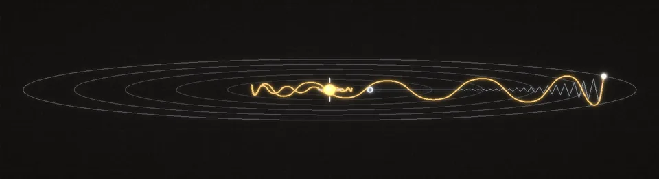On a badly scaled bowl, plain gradient descent zig-zags across the valley and creeps along it. A heavy ball keeps its speed along the floor, where the gradient keeps pointing the same way, overshoots, and settles at the bottom.