Every matrix, symmetric or not, is a rotation, a stretch along perpendicular axes and another rotation. Those stretches, the singular values, measure how much a matrix can grow a vector, bound gradients through a chain of layers, and give the best low-rank approximation.
About 65 minutes
By the end you can
Explain A=UΣV⊤ as rotate, stretch, rotate, and compute it for a 2x2 matrix from A⊤A.
Use ∣Ax∣≤σ1∣x∣ to bound how much a matrix, or a chain of matrices, can grow a vector.
Explain why initialization scales and orthogonal matrices keep singular values near 1.
Build the best rank-k approximation of a matrix and count the numbers it saves.
Look again at a shear, this time S=[1021]. It is triangular, so its eigenvalues are its diagonal entries, 1 and 1, and its spectral radius is 1. If eigenvalues measured stretch, this matrix would stretch nothing. Yet S(0,1)=(2,1), which has length 4+1=5≈2.24, and before the end of this lesson we will find a direction that it stretches by 1+2≈2.41.
Eigenvalues answer the question "which directions survive repeated multiplication, and at what rate?" They do not answer "how much can one multiplication stretch a vector?", which is what you need to know when a gradient passes through a different matrix at every layer or every time step. That second question has its own answer, the singular values.
The road there runs through the previous lesson. Every matrix A, square or not, comes with a symmetric matrix attached, A⊤A, and the spectral theorem applied to it gives the whole answer. The plan: first the picture (every matrix is a rotation, a stretch and a rotation), then how to compute it, then what the largest stretch guarantees, and last how keeping only the biggest stretches compresses a matrix.
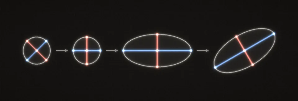
One multiplication stretches different directions by different amounts. For a symmetric matrix the previous lesson gave the full story: a stretch along perpendicular axes. The surprise is that every matrix has such axes. It may also turn the result, so the axes it stretches along are not the axes it lands on.
Follow the unit circle, every vector of length 1, through the three moves. V⊤ turns it, and a turned circle is the same circle. Σ stretches it along the two axes, into an ellipse with half-widths σ1 and σ2. U turns that ellipse into place. So the unit circle goes in and an ellipse comes out, with semi-axes σ1u1 and σ2u2.
Every matrix in three moves: turn, stretch along perpendicular axes, turn again.
For a 2x2 matrix you can check the ellipse directly. Every point of the unit circle is x=costv1+sintv2 for some angle t, because v1,v2 are perpendicular unit vectors. The matrix sends v1 to σ1u1 and v2 to σ2u2 (that is what the three moves do to them), so by linearity Ax=σ1costu1+σ2sintu2. Measured along the perpendicular directions u1,u2, its coordinates are (σ1cost,σ2sint), which trace an ellipse with half-widths σ1 and σ2.
The instrument below draws exactly this for A=[3405]: the white unit circle, its image as a violet ellipse, and the two semi-axes labelled σ1 and σ2, whose lengths are in the readouts. The blue and coral arrows are the columns of A, where ^ and ^ land, and you can drag their tips.
The picture says what the SVD is. To compute it, we need the directions vi that get stretched the most and the least. The symmetric matrix A⊤A finds them.
A⊤A is symmetric. Transpose it, using the transpose rule (which reverses the order) and then (A⊤)⊤=A:
(A⊤A)⊤=A⊤(A⊤)⊤=A⊤A.
It measures stretch. For any x,
x⊤A⊤Ax=(Ax)⊤(Ax)=∣Ax∣2≥0.
In particular, if v is a unit eigenvector of A⊤A with eigenvalue μ, then v⊤A⊤Av=μv⊤v=μ, so μ=∣Av∣2: each eigenvalue of A⊤A is the squared stretch of its own eigenvector, and none is negative.
So take the perpendicular unit eigenvectors v1,v2,… of A⊤A that the spectral theorem promises, and write its eigenvalues, largest first, as σ12≥σ22≥⋯≥0. The numbers σi≥0 are the singular values of A, and ∣Avi∣=σi. For each σi>0 define ui=Avi/σi, the direction vi lands in, scaled to length 1, so that
Avi=σiui.
The ui turn out to be perpendicular to each other too, which is what makes U orthogonal.
Go slower: Why the u vectors are perpendicular, and how A = U Σ Vᵀ follows
Take two indices i and j with σi,σj>0. Write the dot product as a transpose product, use the transpose rule, then A⊤Avj=σj2vj:
The v's are perpendicular unit vectors, so vi⋅vj is 0 when i=j, giving ui⋅uj=0. When i=j it is 1, giving ui⋅ui=σi2/σi2=1.
Now stack the equations Avi=σiui side by side as columns: AV=UΣ, where V has the vi as columns, U the ui, and Σ the σi on its diagonal (the same column argument as AP=PD in the powers lesson). V is orthogonal, so V−1=V⊤, and multiplying both sides on the right by V⊤ gives A=UΣV⊤. (When some σi are zero, or A is not square, U is completed with extra perpendicular unit vectors; they get multiplied by zeros and change nothing.)
Worked example. Take A=[3405], the matrix in the instrument.
Multiply out A⊤A, row of A⊤ by column of A:
A⊤A=[3045][3405]=[9+160+200+200+25]=[25202025].
It has the pattern of [2112] (equal diagonal, equal off-diagonal), so its eigenvectors are (1,1) and (1,−1), and its eigenvalues are 25+20=45 and 25−20=5. As unit vectors, v1=(1,1)/2 and v2=(1,−1)/2.
Take square roots: σ1=45=35≈6.708 and σ2=5≈2.236. These are the 6.71 and 2.24 in the instrument.
Find where each vi lands. Av1=(3+0,4+5)/2=(3,9)/2. Divide by σ1=35, using 2⋅35=310: u1=(3,9)/(310)=(1,3)/10. Likewise Av2=(3−0,4−5)/2=(3,−1)/2, and dividing by σ2=5 gives u2=(3,−1)/10.
Check: u1⋅u2=(1⋅3+3⋅(−1))/10=0, and each has length 10/10=1.
So A stretches the diagonal direction (1,1)/2 the most, by 6.708, onto the direction (1,3)/10, and the other diagonal the least, by 2.236. A quick check: σ1σ2=45×5=225=15, which is ∣detA∣=∣3⋅5−0⋅4∣. In general ∣detA∣ is the product of the singular values, since the two rotations have determinant ±1 and determinants multiply (the rule from module 3).
Two connections to what came before:
For a symmetric matrix, the singular values are the sizes of the eigenvalues. Start from A=QΛQ⊤. For each negative eigenvalue, move its minus sign into the matching column of the left-hand Q: flipping a column keeps that matrix orthogonal, and the middle becomes the diagonal of sizes ∣λi∣. List the eigenvalues largest size first, moving the columns of both Q's to match, and that is an SVD. A symmetric matrix with eigenvalues 3 and −5 has singular values 5 and 3.
PCA is an SVD. If the centered data is X~=UΣV⊤, then X~⊤X~=VΣ⊤U⊤UΣV⊤=VΣ⊤ΣV⊤, and Σ⊤Σ is diagonal with the σi2 on it. So the principal components are the columns of V and the variances are σi2/(n−1). Libraries usually compute PCA this way because it avoids forming X~⊤X~, which squares the numbers and loses precision.
Back to the opening shear. S⊤S=[1201][1021]=[1225] has trace 6 and determinant 5−4=1, so its characteristic equation is λ2−6λ+1=0 and
λ=26±36−4=26±42=3±22.
Their square roots are neater than they look: (2±1)2=2±22+1=3±22, so the singular values are 2+1≈2.414 and 2−1≈0.414. Eigenvalues 1 and 1; singular values 2.414 and 0.414, whose product is (2+1)(2−1)=2−1=1=detS.
To recap: the singular values are the square roots of the eigenvalues of A⊤A; the eigenvectors of A⊤A are the input directions vi, and ui=Avi/σi are where they land. Work one through by hand.
On paperAn SVD by hand
Find the SVD of A=[2−121] by hand, following the worked example in the lesson.
Compute A⊤A, its eigenvalues, and its unit eigenvectors v1,v2.
Take square roots to get σ1≥σ2.
Compute ui=Avi/σi and check that they are perpendicular unit vectors.
Check that σ1σ2=∣detA∣.
Enter σ1 and σ2 below as a column, larger first. Exact forms such as sqrt(8) are accepted, or give 3 decimal places.
Work it on real paper: writing each step is the point. Then check your final answer here and compare your working with the walk-through.
sigma 1 and sigma 2 as a column, larger first (you can type sqrt(8))
One entry per box, top to bottom. 0.25, -2, 3/4 and sqrt(2) all work. Enter moves to the next empty box and checks once all are filled.
The ellipse already says the most useful thing about singular values: no point of the unit circle lands farther out than σ1. Stated for every vector, not just unit ones, that is a bound on growth:
∣Ax∣≤σ1∣x∣for every x,
with equality when x points along v1. For a square matrix the smallest singular value is likewise the least it can stretch a vector: ∣Ax∣≥σn∣x∣.
Go slower: Proof of the bound
Write x in the perpendicular unit basis v1,…,vn: x=c1v1+⋯+cnvn. Because the basis vectors are perpendicular with length 1, the Pythagorean theorem gives ∣x∣2=c12+⋯+cn2.
Apply A, using Avi=σiui: Ax=c1σ1u1+⋯+cnσnun. The ui are also perpendicular unit vectors, so again by Pythagoras
∣Ax∣2=c12σ12+⋯+cn2σn2.
Every σi2 is at most σ12, so
∣Ax∣2≤σ12(c12+⋯+cn2)=σ12∣x∣2.
Take square roots. Equality needs all the weight on σ1, that is, x along v1. Replacing "at most σ12" by "at least σn2" gives the lower bound.
You will meet these numbers under other names. Many sources call σ1 the spectral norm of A and write it ∥A∥2 (double bars are the usual notation for a norm, and the 2 picks this particular one); np.linalg.norm(A, 2) computes it. For a square matrix, the ratio σ1/σn of the most A stretches any direction to the least is the condition numberκ that inverses and systems promised to make precise, and np.linalg.cond computes it exactly this way. For [3405], κ=45/5=9=3.
Eigenvalues are bounded by σ1. An eigenvector is a vector too, so the bound applies to it. If Av=λv, then ∣λ∣∣v∣=∣Av∣≤σ1∣v∣; divide by ∣v∣ to get ∣λ∣≤σ1, and so ρ(A)≤σ1. For symmetric matrices they are equal. For the shear, ρ=1 while σ1≈2.414. For the matrix C=[0.5030.5] in the trap of the powers lesson, ρ=0.5 while σ1≈3.08: the eigenvalues promise decay in the long run, and the large σ1 is what leaves room for the growth in its first steps.
To recap: σ1 is the gain of A, the most it can multiply any length; it goes by the names spectral norm and ∥A∥2; and it is never smaller than the spectral radius. The next exercise shows how far apart the two can be.
Work it outThe largest stretch
What is the largest singular value of A=[02−30]? (Its eigenvalues are ±i6, of modulus about 2.449. That is not the answer.) Enter a single number.
sigma 1
Type a number: 0.25, -2, 3/4 and sqrt(2) all work. Enter checks.
A single bound for a single matrix would be a curiosity. Its real use is that it chains: a vector passing through many different matrices, as activations do through a deep network and gradients do on the way back.
Chains of different matrices. Apply the bound one factor at a time. First ∣A1x∣≤σ1(A1)∣x∣. Then A2 acts on the vector A1x, so ∣A2A1x∣≤σ1(A2)∣A1x∣≤σ1(A2)σ1(A1)∣x∣. And so on down the chain:
∣Ak⋯A2A1x∣≤σ1(Ak)⋯σ1(A2)σ1(A1)∣x∣.
Eigenvalues cannot give a bound like this, because the eigenvalues of a product are not the products of the eigenvalues. For example, [0010] and [0100] are triangular with both eigenvalues 0, yet their product [1000] has the eigenvalue 1.
Gradients in real networks pass through a different matrix at every layer, and in a recurrent network through W⊤ times a different diagonal matrix D of tanh slopes at every step. Backpropagation through time uses exactly this bound. A diagonal matrix stretches by at most its largest entry in size, which for tanh slopes is at most 1. And W⊤ has the same singular values as W: transposing the SVD gives W⊤=VΣ⊤U⊤, another SVD with the same σi. So each step stretches the gradient by at most σ1(W), and if σ1(W)<1 the gradient from k steps back is guaranteed to shrink at least like σ1(W)k. (The bound runs one way only: σ1>1 allows growth but does not force it.)
Initialization. A layer computes Wx. Stack dozens of layers and their stretches multiply, so a network whose weight matrices stretch too much blows its activations up, and one that shrinks too much fades them out. For a random n×n matrix whose entries are independent with mean 0 and variance 1/n, the squared length is preserved on average: the expected value of ∣Wx∣2 is ∣x∣2. That is the reasoning behind the initialization scales in neurons and layers, which adjusts them for the nonlinearity.
Go slower: Why variance 1/n preserves length on average
Entry i of Wx is ∑jWijxj. Its square is a double sum over pairs, ∑j∑lWijWilxjxl. Take the expected value (the average over random draws of W, with x fixed), one term at a time. For j=l the two entries are independent with mean 0, so E[WijWil]=E[Wij]E[Wil]=0. For j=l, E[Wij2]=1/n, the variance. Only the j=l terms survive:
E[(Wx)i2]=j∑n1xj2=n∣x∣2.
There are n entries, each with that expected square, so E[∣Wx∣2]=n⋅∣x∣2/n=∣x∣2.
"On average" hides a spread. This code draws such a matrix with n=256, prints its largest and smallest singular values, and counts how many singular values fall in each range; then it does the same for a random orthogonal matrix.
⌘+Enter runs · edit freelyPython sleeps until you run code
The mean of the squared singular values is close to 1, which is the "on average" promise. But the singular values themselves spread from nearly 0 up to about 2: a random direction keeps its length on average, while some directions are nearly erased and others roughly doubled, at every layer. An orthogonal matrix has every singular value exactly 1, which is why orthogonal initialization is a popular choice for recurrent weight matrices.
To recap: singular values multiply through a chain, so the product of the σ1's bounds any growth, and a network stays well behaved when its layers' singular values sit near 1. Test what singular values do and do not guarantee.
Quick checkWhat singular values guarantee
A 2x2 matrix A has singular values 4 and 0.5. Which statements must be true? Select every one.
The SVD sorts a matrix's stretches from largest to smallest. Throwing away the small ones gives a cheaper matrix that does almost the same job. This is where the best layers in module 3's low-rank instrument came from.
Write the SVD with the outer-product view of matrix multiplication: UΣV⊤ is (column i of UΣ) times (row i of V⊤), summed over i. Column i of UΣ is σiui and row i of V⊤ is vi⊤, so
A=σ1u1v1⊤+σ2u2v2⊤+⋯+σrurvr⊤.
Each term is a rank-one matrix, a column times a row, the kind you met in rank and low-rank updates, and r, the number of nonzero singular values, is the rank of A. (Every output Ax is a combination of u1,…,ur, each ui=Avi/σi is itself an output, and perpendicular vectors are independent, so exactly r dimensions survive.) This is how np.linalg.matrix_rank finds the rank, as that lesson promised: it counts the singular values above a small tolerance, so that rounding noise does not count as a dimension.
The terms come sorted by importance. Keeping the first k gives
Ak=σ1u1v1⊤+⋯+σkukvk⊤.
The error formula is the easy half, and it follows from one fact: rotating or reflecting does not change the Frobenius norm.
Go slower: Why the error is the sum of the dropped squares
Step 1. For an orthogonal Q and any matrix M with matching shape, ∣QM∣F=∣M∣F. The squared Frobenius norm is the sum of the squared lengths of the columns, column j of QM is Q times column j of M, and Q keeps every length. The same holds for ∣MQ∣F, because transposing does not change the sum of squared entries and MQ transposed is Q⊤M⊤, with Q⊤ orthogonal too.
Step 2. Subtract: A−Ak=σk+1uk+1vk+1⊤+⋯+σrurvr⊤=UΣ′V⊤, where Σ′ is Σ with its first k diagonal entries set to zero.
Step 3. By step 1, applied once for U and once for V⊤, ∣A−Ak∣F2=∣Σ′∣F2=σk+12+⋯+σr2. With k=0 this gives ∣A∣F2=σ12+⋯+σr2.
The hard half, that no other rank-k matrix gets closer, needs a longer argument, and we take it on trust.
Worked example. For A=[3405] the best rank-one approximation uses σ1=35, u1=(1,3)/10 and v1=(1,1)/2 from the worked example above. The column (1,3) times the row (1,1) is [1313], and the numbers in front combine as 35/(102)=35/20=35/(25)=3/2:
A1=σ1u1v1⊤=23[1313]=[1.54.51.54.5].
The error is A−A1=[3−1.54−4.50−1.55−4.5]=[1.5−0.5−1.50.5]. Its squared entries add to 2.25+2.25+0.25+0.25=5, which is σ22, as promised.
Storage. An m×n matrix has mn entries. Ak needs only the k columns σiui (length m) and the k rows vi⊤ (length n): k(m+n) numbers. For a 4096×4096 matrix at k=16, that is 16×(4096+4096)=16×8192=131,072 numbers instead of 40962=16,777,216, under 1%. Whether that is a good trade depends entirely on how fast the singular values fall.
The instrument below is the one from module 3, now with the singular values shown. It treats a 16 by 16 picture of a face as a matrix A and shows three pictures side by side: A, its rank-k version Ak, and what is missing, A−Ak. Below them are the slider for k, the layer σkukvk⊤ that was added last, and a bar for every singular value, with the kept ones in lime.
Now build the truncation yourself and look at an error curve for a picture made of two smooth patterns plus noise.
Code itKeep the top singular values
Build truncated-SVD tools and look at an error curve.
rank_k(A, k): keep the k largest singular values from np.linalg.svd and multiply back.
reconstruction_errors(A): the Frobenius errors ∣A−Ak∣F for k=0,1,…,min(m,n), using rank_k.
smallest_rank(A, rel_tol): the smallest k whose error is at most rel_tol times ∣A∣F, computed from the singular values alone with the Eckart-Young formula.
The code at the bottom draws a small image, its rank-2 version, and the error against k.
⌘+Enter runsPython sleeps until you run code
Write your code where the starter says raise NotImplementedError, then press Run tests. Each check says what it expects.
Finally, the confusion this lesson set out to clear up, in your own words.
In your own wordsEigenvalues are not the gain
A colleague says: "All the eigenvalues of my weight matrix are smaller than 1 in size, so no vector can get longer when it passes through this layer." Explain what is wrong, using the difference between eigenvalues and singular values, and say when the colleague's reasoning would be right.


 Every matrix in three moves: turn, stretch along perpendicular axes, turn again.