Mini-batches and linear regression

The last lesson ran gradient descent on losses written as one short formula, whose exact gradient costs almost nothing to compute. A real training loss is an average over a dataset, with one term per example. For a small regression that is 50 terms. For a language model it is trillions of tokens, and computing the exact gradient once would mean a pass over all of them for every single step.

This lesson makes two moves. First, it estimates the gradient from a small random sample of examples, which is how every large model is trained, and it names the optimizer most of them use. Second, it fits linear regression, the one model where gradient descent can be checked against an exact answer, and shows why the scale of the features decides how fast descent gets there.

#Mini-batch gradients

Why can a random handful of examples stand in for the whole dataset? Because the full gradient is an average, and an average can be estimated from a sample.

A training loss is an average over examples: $L(\mathbf{w}) = \frac{1}{N}\sum_{n=1}^{N}\ell_n(\mathbf{w})$, where $\ell_n$ is the loss on example $n$. By the sum rule, its gradient is the average of the per-example gradients, $\nabla L = \frac{1}{N}\sum_{n=1}^{N}\nabla\ell_n$. Computing it exactly costs a pass over all $N$ examples.

So instead, pick a random mini-batch of $B$ examples and average the gradients over just those:

The hat on $\hat{\mathbf{g}}$ marks it as an estimate. A tiny example shows what that estimate does. Suppose a model has one weight and four examples, whose per-example gradients are $1$, $3$, $2$ and $6$. The full gradient is their average, $(1 + 3 + 2 + 6)/4 = 12/4 = 3$. With batches of two examples there are six possible batches:

No batch gives exactly 3, and two of them are off by $1.5$. But the average over all six batches is $(2 + 1.5 + 3.5 + 2.5 + 4.5 + 4)/6 = 18/6 = 3$: exactly the full gradient.

That is what unbiased means: averaged over all the batches you might draw, the estimate equals the true gradient. Any single estimate is noisy. Its variance falls like $1/B$ (averaging $B$ independent random draws divides the variance of one draw by $B$), so its typical error, the standard deviation (the square root of the variance), falls like $1/\sqrt{B}$: four times the batch size halves the typical size of the noise. Each step costs work proportional to $B$ rather than $N$. With $B = 1$ the method is called stochastic gradient descent (SGD); in practice the name is used for any mini-batch size. One pass through the whole dataset is an epoch.

Why does trading exactness for noise pay off? Real datasets are redundant: a thousand examples of a pattern give nearly the same gradient as a million. Many cheap noisy steps make far more progress per unit of compute than a few exact ones. Two side effects follow. The loss curve becomes jagged, so you judge progress by its trend. And with a constant learning rate the weights never settle exactly: near the minimum the gradient is small, but the noise is not, so it keeps them jittering around the minimum. Lowering $\eta$ over the course of training (a schedule) shrinks that jitter.

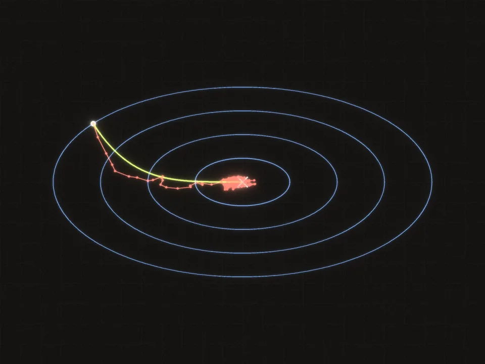Mini-batch steps are noisy but head the right way on average; at a constant learning rate they keep jittering near the bottom.

So far. A mini-batch gradient is the average gradient over a random sample. It is right on average and costs $B/N$ of a full pass, and its noise shrinks like $1/\sqrt{B}$. The price is a jagged loss curve and weights that jitter near the minimum unless the learning rate is lowered.

Check what changes, and what does not, when a full-batch run switches to mini-batches.

#Adam: a step size for each weight

Momentum, from the last lesson, eases badly conditioned valleys by averaging gradients over time. The optimizer most language models are trained with adds a second idea: give every weight its own step size, matched to the size of its own gradients.

Adam (Kingma and Ba; the paper appeared in 2014 and was published at ICLR in 2015) keeps two running averages for every parameter: one of its gradient, like momentum, and one of its squared gradient. Each parameter's step is $\eta$ times its averaged gradient divided by the square root of its averaged squared gradient. That square root is roughly the parameter's typical gradient size.

A small example. One weight gets gradients of about $100$ on every step, another gets gradients of about $0.01$. Plain gradient descent moves them $\eta \times 100$ and $\eta \times 0.01$ per step, so the first moves ten thousand times faster than the second. Adam divides each averaged gradient by its typical size, $100$ and $0.01$, so both move about $\eta$ per step.

That is a cheap, per-coordinate answer to poor conditioning; it helps most when the badly scaled directions line up with individual parameters. Adam and its variant AdamW are the default optimizers for training language models. You will derive and implement Adam in module 6 and use it to train LSTMs in module 8.

#Linear regression, two ways

Linear regression is the one model where you can check gradient descent against an exact answer. It also shows conditioning in its purest form, because its loss is exactly a quadratic bowl.

Its loss is the mean squared error from the gradients lesson, with gradient $\frac{2}{N}\mathbf{X}^\top(\mathbf{X}\mathbf{w} - \mathbf{y})$. At the minimum the gradient is zero. Set it to zero and solve, one move at a time.

1. Start from $\frac{2}{N}\,\mathbf{X}^\top(\mathbf{X}\mathbf{w} - \mathbf{y}) = \mathbf{0}$.

2. Multiply both sides by $\frac{N}{2}$: $\mathbf{X}^\top(\mathbf{X}\mathbf{w} - \mathbf{y}) = \mathbf{0}$.

3. Multiply out the bracket: $\mathbf{X}^\top\mathbf{X}\,\mathbf{w} - \mathbf{X}^\top\mathbf{y} = \mathbf{0}$.

4. Move $\mathbf{X}^\top\mathbf{y}$ to the right side. The result is the normal equations:

   $$\mathbf{X}^\top\mathbf{X}\,\mathbf{w} = \mathbf{X}^\top\mathbf{y}.$$

When the columns of $\mathbf{X}$ are independent, $\mathbf{X}^\top\mathbf{X}$ is invertible and this has exactly one solution. In code, solve it with np.linalg.solve rather than by forming an inverse, as in module 3.

Take the three points from the gradients lesson: feature values $1,\allowbreak 2,\allowbreak 3$ with targets $1,\allowbreak 2,\allowbreak 2$, and $\mathbf{X} = \begin{bmatrix} 1 & 1 \\ 1 & 2 \\ 1 & 3 \end{bmatrix}$, whose column of ones carries the bias.

1. $\mathbf{X}^\top\mathbf{X}$. Dot the columns of $\mathbf{X}$ with each other: ones with ones gives $1 + 1 + 1 = 3$, ones with the feature gives $1 + 2 + 3 = 6$, the feature with itself gives $1 + 4 + 9 = 14$. So $\mathbf{X}^\top\mathbf{X} = \begin{bmatrix} 3 & 6 \\ 6 & 14 \end{bmatrix}$.
2. $\mathbf{X}^\top\mathbf{y}$. Dot each column with $\mathbf{y} = (1,\allowbreak 2,\allowbreak 2)$: $(1 + 2 + 2,\allowbreak \ 1 + 4 + 6) = (5,\allowbreak 11)$.
3. Solve. The determinant is $3 \times 14 - 6 \times 6 = 42 - 36 = 6$, so the inverse is $\frac{1}{6}\begin{bmatrix} 14 & -6 \\ -6 & 3 \end{bmatrix}$ (swap the two diagonal entries, negate the other two, divide by the determinant, as in module 3), and $\mathbf{w} = \frac{1}{6}\,(14 \times 5 - 6 \times 11,\allowbreak \ -6 \times 5 + 3 \times 11) = \frac{1}{6}(70 - 66,\allowbreak \ -30 + 33) = \frac{1}{6}(4,\allowbreak 3) = \left(\tfrac{2}{3},\allowbreak \tfrac{1}{2}\right)$.

The best line is $\hat{y} = \tfrac{2}{3} + \tfrac{1}{2}x$. Its predictions are $\tfrac{7}{6}$, $\tfrac{5}{3}$ and $\tfrac{13}{6}$, so its residuals are $\mathbf{r} = (\tfrac{1}{6},\allowbreak -\tfrac{1}{3},\allowbreak \tfrac{1}{6})$, and $\mathbf{X}^\top\mathbf{r} = (\tfrac{1}{6} - \tfrac{1}{3} + \tfrac{1}{6},\allowbreak \ \tfrac{1}{6} - \tfrac{2}{3} + \tfrac{3}{6}) = (0,\allowbreak 0)$: the gradient is zero, as it must be at the minimum.

Now gradient descent. The Hessian is the Jacobian of the gradient. The gradient $\frac{2}{N}(\mathbf{X}^\top\mathbf{X}\,\mathbf{w} - \mathbf{X}^\top\mathbf{y})$ is a matrix times $\mathbf{w}$ plus a constant, so its Jacobian is that matrix: the Hessian is $\frac{2}{N}\mathbf{X}^\top\mathbf{X}$ at every point. The loss is exactly a quadratic bowl, and everything in the last lesson applies without approximation. For the three points, $\mathbf{H} = \frac{2}{3}\begin{bmatrix} 3 & 6 \\ 6 & 14 \end{bmatrix} = \begin{bmatrix} 2 & 4 \\ 4 & \tfrac{28}{3} \end{bmatrix}$, with eigenvalues about $11.09$ and $0.24$ (the roots of $\lambda^2 - \tfrac{34}{3}\lambda + \tfrac{8}{3} = 0$, whose coefficients are the trace $2 + \tfrac{28}{3} = \tfrac{34}{3}$ and the determinant $2 \times \tfrac{28}{3} - 4 \times 4 = \tfrac{56}{3} - \tfrac{48}{3} = \tfrac{8}{3}$, as in module 4): a condition number of $11.09 / 0.24 \approx 46$. Even this tiny problem is a narrow valley.

The scale of the features sets the curvatures. If one feature takes values in the thousands and another in single digits, $\mathbf{X}^\top\mathbf{X}$ has one enormous eigenvalue and one small one, the condition number is huge, and gradient descent crawls. Standardizing each feature (subtract its mean, divide by its standard deviation) makes the curvatures similar. It is conditioning, done by hand.

The code below fits a bias and a single feature ranging from 0 to 10: 50 noisy points around the line $y = 2 + 0.5x$. It solves the normal equations, prints the Hessian's eigenvalues, runs 2,000 steps of full-batch gradient descent at half the stability limit, and then repeats the fit with the feature standardized. Even this mild mismatch in scale gives a condition number above 100.

The closed form is $(1.8787,\allowbreak 0.5262)$: bias about $1.88$, slope about $0.53$. After 100 steps of descent the slope is too large by about a quarter and the bias is only about half its final value; after 2,000 steps gradient descent agrees with the closed form to four decimals. The flat direction, which mixes the bias with the slope, is what takes so long.

Why standardizing fixes it

Standardizing the feature fixes it completely: both Hessian eigenvalues become exactly 2, the bowl is perfectly round, and a single step at $\eta = 1/\lambda = 0.5$ lands on the answer. (The weights differ from the ones above because the feature is now measured in different units; they describe the same line.)

Subtracting the mean matters as much as dividing by the standard deviation. A feature that is always positive, like this $x$, overlaps with the column of ones, so the bias and the slope compete to explain the same thing, and that overlap is the flat, mixed direction. Centering makes the two columns perpendicular. On this data, dividing by the standard deviation alone brings the condition number from 161 to about 26, subtracting the mean alone brings it to about 8.5, and both together bring it to 1.

In short. The normal equations give linear regression's answer in one solve. Gradient descent reaches the same answer, at a pace set by the condition number of $\frac{2}{N}\mathbf{X}^\top\mathbf{X}$, and standardizing the features brings that condition number down toward 1.

Now write both methods yourself: the closed form, and mini-batch descent that should land close to it.

The next exercise closes the loop between theory and practice: predict the learning-rate limit from the Hessian, then watch a sweep of learning rates confirm it, and see what standardizing does to the condition number.

Finally, diagnose a colleague's slow model with everything from this lesson and the last.