With many inputs, the derivative becomes a vector with one entry per input. It points in the direction the function climbs fastest, and every training step moves against it.
About 65 minutes
By the end you can
Compute partial derivatives and assemble them into a gradient.
Use the directional derivative ∇f⋅u to explain why the gradient points uphill fastest and is perpendicular to contour lines.
Derive the gradients of w⋅x, ∣x∣2, x⊤Ax and the mean squared error of linear regression.
Write a numerical gradient for any function and use it to check an analytic gradient.
Now the model has two weights, and the loss L(w1,w2) is a landscape: a height above every point of a plane. You are standing somewhere on it in thick fog. You cannot see the valley, but you can feel the ground under your feet. Take a small step east and notice how much you drop. Take a small step north and notice again.
Those two numbers turn out to be enough. From them alone you can work out the slope in every other direction, including which way is steepest downhill and how steep it is. The pair is called the gradient. A language model's loss is a landscape over billions of weights, and its gradient has billions of entries, but it is built and read exactly the way this lesson builds and reads the two-entry version.
The lesson goes in five steps: measure one input at a time (partial derivatives), combine them into a forecast, find which way is uphill, work out the gradients of the pieces that models are built from, and assemble those pieces into the gradient of linear regression's loss.
With one input there was one slope. With two inputs there is a slope for each, and the simplest way to measure one of them is to keep the other input still. For a function of several inputs, the partial derivative with respect to one input is the ordinary derivative you get by holding every other input fixed. It is written with a curly ∂ to signal that the others are frozen: ∂x∂f is read "the partial of f with respect to x".
Take f(x,y)=x2y+3y at the point (2,1), where f=22×1+3×1=4+3=7.
For ∂x∂f, treat y as a constant. Then x2y is a constant times x2, with derivative 2x⋅y=2xy, and 3y does not change with x at all. So ∂x∂f=2xy, which is 2×2×1=4 at (2,1).
For ∂y∂f, treat x as a constant. Then x2y is the constant x2 times y, with slope x2, and 3y has slope 3. So ∂y∂f=x2+3, which is 4+3=7 at (2,1).
You can check both by experiment. Nudge x alone: f(2.01,1)=2.012+3=4.0401+3=7.0401, a change of 0.0401 for a nudge of 0.01, a rate of 4.01. Nudge y alone: f(2,1.01)=4×1.01+3×1.01=4.04+3.03=7.07, a change of 0.07, a rate of exactly 7, because with x held fixed f is a straight line in y.
The gradient collects all the partial derivatives into one vector:
∇f=(∂x1∂f,∂x2∂f,…,∂xn∂f).
The symbol ∇ is read "grad" (or "nabla"). Here ∇f(2,1)=(4,7). When a function has several groups of inputs, a subscript says which ones we differentiate with respect to: ∇wL is the gradient of the loss with respect to the weights only, with the data held fixed.
In one dimension the derivative gave a forecast, f(x+h)≈f(x)+f′(x)h. The gradient gives the same kind of forecast when every input moves at once. Take a small step h=(h1,…,hn). Each input's nudge contributes its partial derivative times its size, and the contributions add up:
f(x+h)≈f(x)+∂x1∂fh1+⋯+∂xn∂fhn=f(x)+∇f(x)⋅h.
The last form is a dot product, from module 1: the gradient dotted with the step.
With our example, step from (2,1) to (2.1,0.9), so h=(0.1,−0.1):
f(2.1,0.9)≈7+4×0.1+7×(−0.1)=7+0.4−0.7=6.7.
The true value is 2.12×0.9+3×0.9=3.969+2.7=6.669, so the forecast is off by 0.031.
Go slower: Why the separate contributions add
Take two inputs. Get from (x,y) to (x+h1,y+h2) in two moves, first changing y and then changing x. Adding and subtracting the halfway value f(x,y+h2) splits the total change into two pieces:
f(x+h1,y+h2)−f(x,y)=only x changesf(x+h1,y+h2)−f(x,y+h2)+only y changesf(x,y+h2)−f(x,y).
The second piece changes only y, so by the one-dimensional approximation it is about ∂y∂f(x,y)h2.
The first piece changes only x, at height y+h2, so it is about ∂x∂f(x,y+h2)h1.
When the partial derivatives change smoothly from point to point (true for every function in this course apart from kinks like ReLU's corner), ∂x∂f(x,y+h2) is close to ∂x∂f(x,y) for small h2. So the total change is about ∂x∂fh1+∂y∂fh2.
With n inputs, make n moves, one coordinate at a time, and the same argument gives one term per coordinate.
So far. A partial derivative measures one input's effect with the others frozen. The gradient stacks them into a vector, and the gradient dotted with a small step forecasts how much the function changes.
Try both on one function: find its gradient at a point, then use it to forecast a nearby value.
On paperA gradient and a prediction
Let f(x,y)=x2y−3xy+y2.
Find ∂x∂f and ∂y∂f, and evaluate the gradient at (2,−1).
Use the linear approximation to estimate f(2.1,−0.9). You will need f(2,−1).
To check your work, enter ∂x∂f and ∂y∂f at (2,−1) and then the estimate, in that order, as decimals.
Work it on real paper: writing each step is the point. Then check your final answer here and compare your working with the walk-through.
∂f/∂x and ∂f/∂y at (2, -1), then the estimate
One entry per box, top to bottom. 0.25, -2, 3/4 and sqrt(2) all work. Enter moves to the next empty box and checks once all are filled.
Training wants the direction in which the loss falls fastest. The gradient answers that, and the reason takes one line of algebra plus the geometry of the dot product.
Stand at x and choose a direction, given as a unit vector u (a vector of length 1). Walk a small distance t along it, so the step is h=tu. The forecast from the last section says
f(x+tu)≈f(x)+∇f(x)⋅(tu)=f(x)+t∇f(x)⋅u.
So the function changes by about ∇f⋅u per unit of distance walked. That rate is the slope in the direction u, called the directional derivative:
Duf=∇f⋅u.
The partial derivatives are the special cases u=(1,0) and u=(0,1). Now use the geometric reading of the dot product from module 1: ∇f⋅u=∣∇f∣∣u∣cosθ=∣∇f∣cosθ, where θ is the angle between the gradient and your direction, and ∣u∣=1. Three facts follow.
Uphill fastest along the gradient.cosθ is largest, 1, at θ=0. The steepest slope available is ∣∇f∣, the length of the gradient.
Downhill fastest against it. At θ=180° the slope is −∣∇f∣. This is the direction gradient descent steps in.
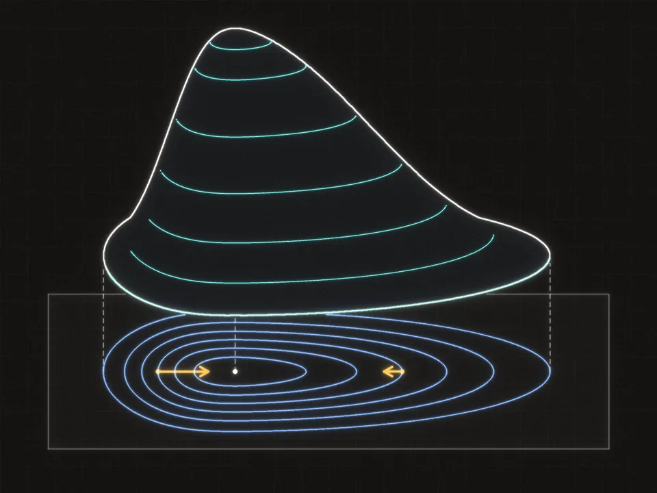
Level along the contours. At θ=90° the slope is zero: to first order, the function does not change. A contour line (a curve of constant height, as on a hiking map) runs in exactly those directions. So the gradient is perpendicular to the contour lines.
The gradient is an arrow on the map, not on the hillside: it crosses each contour at a right angle and grows where the lines crowd together.
A worked example. Let f(x,y)=x2+2y2 at (3,1), where f=9+2=11. The partial derivatives are 2x and 4y, so the gradient is (2×3,4×1)=(6,4), with length 62+42=36+16=52≈7.21. Here is the slope ∇f⋅u in five directions:
direction u
slope ∇f⋅u
east, (1,0)
6×1+4×0=6
north, (0,1)
6×0+4×1=4
diagonal, (1,1)/2
(6+4)/2=10/2≈7.07
along the gradient, (6,4)/52
(36+16)/52=52≈7.21
perpendicular, (−4,6)/52
(−24+24)/52=0
The last row's direction comes from swapping the gradient's two entries and flipping the sign of one: (6,4) becomes (−4,6), and the dot product 6×(−4)+4×6 is then zero by construction. No direction beats 7.21. The last direction, (−4,6), is the way the contour x2+2y2=11 runs through (3,1): walk that way and, to first order, you stay at height 11.
The widget shows the same facts on a different surface, L=21x2+5y2: a long valley whose minimum is at the origin. It is drawn from above as a contour map. The pink lines join points of equal loss, the shading darkens toward low loss, and the lime cross marks the minimum. The small amber arrows show the gradient's direction on a grid of points. The white probe is the point the readouts describe: its own amber arrow is ∇L there, and the dashed white line through it follows the contour.
Here is the cosine law measured directly. The code walks around the point (3,1) of f=x2+2y2, one direction every 5 degrees, estimates the slope in each direction with a central difference from derivatives by experiment, and plots it next to the prediction ∇f⋅u=∣∇f∣cosθ.
⌘+Enter runs · edit freelyPython sleeps until you run code
The two curves lie on top of each other: a cosine wave with amplitude ∣∇f∣≈7.21, peaking in the gradient's direction (about 33.7°; the nearest direction tried is 35°).
So far. The slope in any unit direction u is ∇f⋅u=∣∇f∣cosθ. So the gradient points up the steepest slope, its length is that slope, and it crosses every contour at a right angle. Gradient descent walks the opposite way.
Check the three facts on a gradient of your own, including the classic slip of mixing up a direction with a step.
Quick checkSteepest way down
At a point, the gradient of a loss is ∇L=(3,−4). In which unit direction does the loss decrease fastest, and at what rate (change in loss per unit distance)?
Choose one answer, then check.
Now put the whole argument of this section into your own words, starting from the forecast and ending at the contour lines.
In your own wordsWhy the gradient points uphill
Explain, without assuming the result, why the gradient points in the direction of steepest ascent, why its length is the steepest slope, and why it is perpendicular to contour lines. Build the argument from the directional derivative.
Most gradients in machine learning are assembled from a few pieces, so it pays to know those pieces by heart. A reliable way to find a gradient you do not know has three moves: write the function as a sum over indices, take the partial derivative with respect to a single entry, say wk, and then recognize the resulting list of numbers as a vector expression.
A dot product with a fixed vector.f(w)=w⋅x=w1x1+⋯+wnxn. Only the term wkxk involves wk, so ∂wk∂f=xk. With two entries: ∂w1∂f=x1 and ∂w2∂f=x2, and stacking them gives back x. In general,
∇w(w⋅x)=x.
This is the gradient of a neuron's weighted sum with respect to its weights: the input itself. In module 6 it becomes the rule that each weight's gradient is the input it saw times the error signal arriving from above.
A squared length.f(x)=∣x∣2=x12+⋯+xn2. Only the term xk2 involves xk, so ∂xk∂f=2xk, and
∇∣x∣2=2x.
This is the one-dimensional rule x2↦2x, entry by entry. The gradient points straight away from the origin, which fits the circular contours of this function.
A quadratic form. For a square matrix A, let f(x)=x⊤Ax. (The transpose x⊤ turns the column x into a row, so the result is a single number: the dot product of x with Ax.) Written as a double sum, f=∑i∑jxiAijxj, and its gradient is
∇(x⊤Ax)=(A+A⊤)x,which is 2Ax when A is symmetric.
The symmetric case is the matrix version of ax2↦2ax.
Go slower: The gradient of a quadratic form, index by index
Step 1, differentiate one term. Each term xiAijxj contains the product xixj. By the product rule, its partial derivative with respect to xk is
Aij(∂xk∂xixj+xi∂xk∂xj),
where ∂xk∂xi is 1 when i=k and 0 otherwise.
Step 2, sum over all terms. In the first part only the terms with i=k survive; in the second only those with j=k:
∂xk∂f=j∑Akjxj+i∑xiAik.
Step 3, recognize the sums. The first sum is entry k of Ax (row k of A dotted with x). The second is ∑i(A⊤)kixi, because Aik=(A⊤)ki, so it is entry k of A⊤x.
Step 4, stack the entries.∇f=Ax+A⊤x=(A+A⊤)x. If A=A⊤, this is 2Ax.
A worked example with the symmetric matrix A=[2113] and x=(1,2).
Multiply.Ax=(2×1+1×2,1×1+3×2)=(4,7).
The value.f=x⋅Ax=1×4+2×7=18.
The gradient.A is symmetric, so ∇f=2Ax=(8,14).
Check by multiplying out: f=2x12+2x1x2+3x22, so ∂x1∂f=4x1+2x2=4+4=8 and ∂x2∂f=2x1+6x2=2+12=14.
Quadratic forms matter because every smooth loss looks like one near its minimum. That fact runs the whole analysis of gradient descent two lessons from now.
The next exercise uses a matrix that is not symmetric, where the shortcut 2Ax gives the wrong answer.
Work it outA quadratic form that is not symmetric
Let A=[1023] and f(x)=x⊤Ax. Find ∇f at x=(1,1). Enter it as a column: ∂x1∂f on top, ∂x2∂f below.
∇f(1, 1)
One entry per box, top to bottom. 0.25, -2, 3/4 and sqrt(2) all work. Enter moves to the next empty box and checks once all are filled.
Linear regression is the first model you will train in this course, and its gradient has the shape every layer's weight gradient will have: the inputs, transposed, times the errors. It is built from the pieces above plus the chain rule.
Linear regression predicts a number from d features with a weight vector w. Stack N examples as the rows of a matrix X with shape N×d (the row-batch convention from module 2), and their targets in a vector y of length N. The predictions are Xw, one per example. The residuals (prediction minus target) are r=Xw−y, and the loss is the mean squared error
L(w)=N1n=1∑Nrn2=N1∣Xw−y∣2.
Its gradient is
∇wL=N2X⊤(Xw−y).Go slower: Deriving the regression gradient
Step 1, one residual. Residual n is rn=∑kXnkwk−yn. Only the term Xnkwk involves wk, so ∂wk∂rn=Xnk.
Step 2, one squared residual (chain rule). The outer function is squaring, with slope 2rn; the inner function is rn. So ∂wk∂(rn2)=2rn∂wk∂rn=2rnXnk.
Step 3, average over examples (sum rule).
∂wk∂L=N1n=1∑N2rnXnk=N2n=1∑N(X⊤)knrn,
where the last form only renames Xnk as (X⊤)kn.
Step 4, recognize the matrix product. The last sum is row k of X⊤ dotted with r: entry k of X⊤r. So ∇wL=N2X⊤r=N2X⊤(Xw−y).
Shape check.X⊤ is d×N and r has length N, so the result has length d: one entry per weight, as a gradient must.
A worked example with three points. Let
X=111123,y=122,w=[01].
The column of ones is a standard trick: its weight w1 acts as the bias (the intercept), so the model is y^=w1+w2x with feature values x=1,2,3.
Predictions.Xw=(0+1,0+2,0+3)=(1,2,3).
Residuals.r=(1−1,2−2,3−2)=(0,0,1).
Loss.L=31(02+02+12)=31.
X⊤r. Row 1 of X⊤ is (1,1,1) and row 2 is (1,2,3), so X⊤r=(0+0+1,0+0+3)=(1,3).
Gradient. Multiply by N2=32:
∇wL=32(1,3)=(32,2).
Read it: only the third example is wrong, and it is over-predicted, so both partial derivatives are positive and the gradient says "decrease both weights". The slope's entry is three times the bias's because that example's feature value is 3.
Now derive the same gradient for a line fit of your own, as sums over the points, and evaluate it.
On paperOne gradient for a line fit
Fit y^=wx+b to three points (x,y): (0,1), (1,3) and (2,4), with loss L=31∑n(y^n−yn)2.
Write X (one row per point, with a column of ones for the bias) and derive ∂w∂L and ∂b∂L as sums over the points.
Evaluate the loss and both partial derivatives at w=1, b=1.
Which way should each parameter move?
To check your work, enter L, ∂w∂L and ∂b∂L at w=1, b=1, in that order, as fractions (such as 5/6) or decimals to 3 places.
Work it on real paper: writing each step is the point. Then check your final answer here and compare your working with the walk-through.
L, ∂L/∂w and ∂L/∂b at w = 1, b = 1
One entry per box, top to bottom. 0.25, -2, 3/4 and sqrt(2) all work. Enter moves to the next empty box and checks once all are filled.
Deriving gradients by hand is error-prone, so every gradient you derive in this course gets checked against a numerical one: the central differences from the previous lesson, applied one coordinate at a time. Nudge one entry up by h, then down by h, divide the difference in outputs by 2h, put the entry back, and move to the next one. Build that checker now; you will use the idea in every later module.
Code itA gradient checker
Write a gradient checker you can reuse, and two analytic gradients to check with it.
num_grad(f, x, h=1e-5): the central-difference gradient of a scalar function f at an array x of any shape. It must not change x, and it must work when x is a list of integers.
grad_quadratic(A, x): the exact gradient of x⊤Ax for a square A that need not be symmetric.
mse_loss_and_grad(X, y, w): the mean squared error of the predictions X @ w, and its gradient N2X⊤(Xw−y).
The tests compare your analytic gradients with numerical ones, which is how every backward pass in this course gets checked.
⌘+Enter runsPython sleeps until you run code
Write your code where the starter says raise NotImplementedError, then press Run tests. Each check says what it expects.
For more practice, work through a few generated gradients: partial derivatives, directional derivatives, quadratic forms and a small regression loss.
Practice setGradient reps
3 correct in a row completes the set. A miss starts the count again.
Let f(x,y)=−x2+y2+2x−2y. Find the directional derivative Duf=∇f⋅u at (x,y)=(1,0) in the direction of the unit vector u=(0,−1). Give the exact value.
D_u f
Type a number: 0.25, -2, 3/4 and sqrt(2) all work. Enter checks.


 The gradient is an arrow on the map, not on the hillside: it crosses each contour at a right angle and grows where the lines crowd together.