Activations and initialization

A lamp has two switches, and it should light up when exactly one of them is on. Write the switches as $x_1,\allowbreak x_2 \in \{0,\allowbreak 1\}$ (each is 0 for off or 1 for on). The four cases are $(0,\allowbreak 0) \to 0$, $(0,\allowbreak 1) \to 1$, $(1,\allowbreak 0) \to 1$ and $(1,\allowbreak 1) \to 0$. This is the exclusive or, XOR.

The last lesson ended with two facts that make this lamp hard. One neuron draws one straight line. And a stack of layers without a bend is still one layer, so it still draws one straight line. Step 6 of its walkthrough showed the result: on XOR data, a single neuron gave up at a 50/50 guess. This lesson proves that no line can do better, looks closely at the bends in common use, shows how a hidden layer uses one to get around the problem, and ends with the question every training run starts with: what should the weights be before any learning has happened?

#No single line can split XOR

Why prove it, when the widget already failed? Because a failed training run could mean a bad learning rate or bad luck. A proof says that no choice of weights works, so something in the network has to change.

Suppose a neuron had $z = w_1x_1 + w_2x_2 + b$ positive exactly on the two "on" inputs. Write down what each input demands:

1. $(0,\allowbreak 1)$ is on, so $z = w_2 + b > 0$.
2. $(1,\allowbreak 0)$ is on, so $z = w_1 + b > 0$.
3. Adding lines 1 and 2: $w_1 + w_2 + 2b > 0$.
4. $(0,\allowbreak 0)$ is off, so $z = b \le 0$.
5. $(1,\allowbreak 1)$ is off, so $z = w_1 + w_2 + b \le 0$.
6. Adding lines 4 and 5: $w_1 + w_2 + 2b \le 0$.

Lines 3 and 6 contradict each other, so no choice of weights works. The picture behind the algebra: $z$ changes at a steady rate along any straight segment, so its value at the center of the square, $(0.5,\allowbreak 0.5)$, is the average of its values at the two ends of either diagonal. The "on" diagonal, from $(0,\allowbreak 1)$ to $(1,\allowbreak 0)$, makes that average positive; the "off" diagonal, from $(0,\allowbreak 0)$ to $(1,\allowbreak 1)$, makes it zero or negative. Both cannot be true. (Lines 3 and 6 are exactly twice the value at the center.)

#The activation functions

The fix, as the next section shows, is a bend between two layers. Before using one, look at the bends in common use. Two things matter about each: its shape, which decides what the network can represent, and its slope $\phi'$, which decides how well it trains, because every gradient flowing backward through a unit gets multiplied by that slope (backpropagation makes this precise).

The widget answers one question: what does each activation do to its input, and how steep is it there? It plots four functions of one input $x$: sigmoid in teal, tanh in violet, ReLU in coral and GELU in lime, with their slopes as dashed curves of the same colors. The dashed blue vertical line marks the current $x$ (drag it, or use the $x$ slider); the table in the side panel gives each function's value and slope there, with an amber bar for the size of the slope. One function at a time is focused (drawn thicker, with its tangent line in amber), and hatched bands mark where the focused function's slope is below 0.05, so a gradient passing back keeps less than 5% of its size. The live note turns the focused slope into what happens to a gradient.

Here are the four in words, with the facts the widget just showed.

• Sigmoid, $\sigma(z) = \frac{1}{1 + e^{-z}}$, outputs values in $(0,\allowbreak 1)$. Its slope $\sigma(z)(1 - \sigma(z))$ is at most $0.25$, at $z = 0$, and nearly zero once $|z|$ is above about 5. It is the right choice when you need a probability or a soft on-off switch, which is why every LSTM gate in module 8 is a sigmoid.
• Tanh outputs values in $(-1,\allowbreak 1)$ and is centered at zero. It is a rescaled sigmoid, $\tanh(z) = 2\sigma(2z) - 1$ (at $z = 0$: $2(0.5) - 1 = 0$), with slope $1 - \tanh^2(z)$, which peaks at 1. Centering matters because of what the next layer sees. If every input to a neuron is positive, as sigmoid outputs are, then (as backpropagation will show) the gradients of all its weights for one example share one sign. Its weights can then only all rise or all fall together on that example, and training zig-zags. Tanh outputs of both signs avoid this, which suits hidden layers.
• ReLU, $\max(0,\allowbreak z)$, has slope exactly 1 for $z > 0$ and 0 for $z < 0$. At $z = 0$ it has a corner, where code picks one of the two slopes.
• GELU, $z\,\Phi(z)$, where $\Phi$ is the cumulative distribution function of a standard normal variable (the probability that such a variable is below $z$). For large positive $z$, $\Phi(z)$ is nearly 1 and GELU is nearly $z$; for very negative $z$, $\Phi(z)$ is nearly 0 and so is GELU. In between it dips to about $-0.17$ near $z = -0.75$.

Why ReLU won for deep networks. A gradient passing backward through $k$ layers is multiplied by $k$ slopes, one per layer. With sigmoids each slope is at most $0.25$, so across ten layers the slopes alone multiply the gradient by at most $0.25^{10} \approx 9.5 \times 10^{-7}$, a loss the weights would have to make up. That is the vanishing gradient problem in its simplest form, and module 7 meets it again through time. A ReLU unit that is on passes the gradient back unchanged, so deep stacks of ReLUs train far more readily. It is also cheap to compute. AlexNet, the convolutional network that won the 2012 ImageNet competition, used ReLUs; its authors reported that in a smaller test network, ReLUs reached a given training error six times faster than tanh units. The cost is dead units: a ReLU whose input is negative for every example outputs 0 and passes back no gradient (step 4 of the walkthrough), so its incoming weights stop learning and it can stay off for good. Variants such as the leaky ReLU keep a small slope for negative inputs to avoid this.

GELU (Hendrycks and Gimpel, 2016) became the default in transformers: BERT and GPT-2 use it. Many recent language models, such as the Llama family, use a gated design called SwiGLU instead, in which one linear projection, passed through a smooth ReLU-like curve, multiplies a second projection entry by entry. The details differ; the job is the same: bend space between two matrix multiplies.

Put a number on the vanishing gradient before moving on.

To recap: every activation is a fixed bend, and its slope is a toll every gradient pays on the way back. Sigmoid and tanh saturate on both sides; ReLU passes gradients untouched when on and blocks them when off; GELU is a smooth ReLU.

#Bending space until a line works

Now use a bend to solve the lamp. The trick is not to find a cleverer line in the $(x_1,\allowbreak x_2)$ plane, since the first section proved there is none, but to move the points first. Use two ReLU hidden units that both look at $x_1 + x_2$, the second with a threshold of 1, and an output that combines them:

Work through the four inputs. For $(1,\allowbreak 1)$, for example: $x_1 + x_2 = 2$, so $h_1 = \operatorname{ReLU}(2) = 2$ and $h_2 = \operatorname{ReLU}(2 - 1) = 1$, and $\hat{y} = 2 - 2(1) = 0$.

It computes XOR exactly. Look at the $(h_1,\allowbreak h_2)$ column: the hidden layer sends the two "on" inputs to the same point $(1,\allowbreak 0)$ and moves $(1,\allowbreak 1)$ out to $(2,\allowbreak 1)$. In the new coordinates the three distinct points are $(0,\allowbreak 0)$, $(1,\allowbreak 0)$ and $(2,\allowbreak 1)$, and a straight line such as $h_1 - 2h_2 = 0.5$ separates them: the left side $h_1 - 2h_2$ is $0$ at $(0,\allowbreak 0)$, $1$ at $(1,\allowbreak 0)$ and $2 - 2 = 0$ at $(2,\allowbreak 1)$, so only $(1,\allowbreak 0)$ lands above 0.5. The hidden layer folded the plane so that the problem became linear, and the output neuron finished the job with a line.

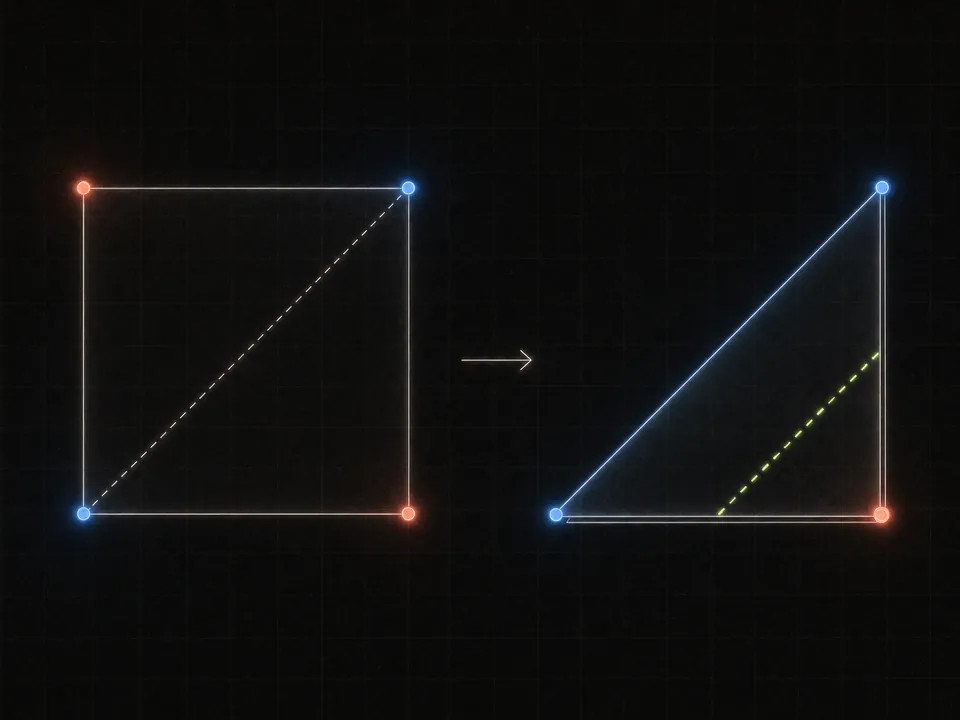Fold the square along the blue diagonal and the two coral corners meet. After the fold, one straight cut separates them from the blue ones.

Now watch training find such coordinates on its own. The widget below trains a 2-2-1 network with tanh hidden units on noisy XOR data: four clusters of 50 points around $(\pm 0.6,\allowbreak \pm 0.6)$, coral where exactly one coordinate is positive. The big plot shows the data over the network's prediction, as in the last lesson. Under it, the network is drawn as tiles: each neuron is a small square showing its own output over the same plane (blue low, coral high), with a thin line where its $z = 0$, and each weight is a line between tiles, coral for positive and blue for negative, thicker when larger. Hover over or tap a tile and the text below the network says what that neuron computes, with its live numbers, while its line appears on the big plot in lime dashes. Because the hidden layer has exactly two units, a switch above the plot can also show hidden space: every point drawn at its two hidden outputs $(h_1,\allowbreak h_2)$ instead of $(x_1,\allowbreak x_2)$.

How far does this go? The universal approximation theorem (Cybenko, 1989, for sigmoid units; Hornik, Stinchcombe and White, 1989, more generally) says that a network with a single hidden layer and enough units can approximate any continuous function on a closed, bounded region as closely as you like. Later work showed that any activation that is not a polynomial will do, ReLU included. State it honestly, because it is often oversold:

• It says such weights exist. It does not say gradient descent will find them.
• It says nothing about how many units are needed, and for some functions a single hidden layer needs astronomically many. Deep networks can represent some functions with far fewer units than shallow ones, which is one reason depth pays off in practice.
• It says nothing about generalization: fitting the training points is not the same as being right on new ones. That is the subject of the training lesson.

You now have the whole argument for why networks need a bend. Put it in your own words.

To recap: no line splits XOR in the input plane, but a hidden layer with a bend moves the points into new coordinates where one does. Training finds those coordinates by itself, and with more units a single hidden layer can approximate far more than XOR.

#Where to start: initialization

Every training run starts from some choice of weights and improves it. The widget above started from small random weights, and it trained. Two things about that starting point decide whether training can work at all.

Not all equal, and certainly not all zero. Suppose every weight starts at the same value, both in the hidden layer and in the layer that reads it. Then every hidden unit computes the same function of the input, produces the same output, sends it on through the same outgoing weights, and (as you will see in backpropagation) receives the same gradient. They take identical steps and stay identical forever: 64 hidden units behave like one. Starting every weight and bias at exactly zero is worse. With $\tanh$ hidden units, every hidden output is then $\tanh(0) = 0$. The gradient of $\mathbf{W}_2$ is built from the hidden outputs, so $\mathbf{W}_2$ gets no gradient. The gradient reaching the hidden layer passes back through $\mathbf{W}_2 = \mathbf{0}$, so the first layer gets none either. Only the output bias ever moves. Random starting weights break this symmetry.

Not too big, not too small. Each layer multiplies its input by a matrix. Module 4 showed that a random $n \times n$ matrix with entries of variance $1/n$ preserves squared length on average, and that a matrix stretches a vector by at most its largest singular value, so a stack of layers can stretch by at most the product of theirs. Get the scale wrong by a constant factor and after 20 layers the signal has been multiplied or divided by that factor about 20 times. Too small and the activations fade toward zero; too large and tanh units saturate at $\pm 1$, where (step 3 of the activation walkthrough) their slope is nearly zero, so the gradients die on the way back.

The right scale comes from one short calculation about the variance of a pre-activation, its average squared size. The box below does it one move at a time.

Run the experiment. The code pushes 200 random inputs through 20 layers of width 200 and plots the root-mean-square activation (the square root of the average squared activation, a typical size) after each layer, for several weight scales.

Read the printout line by line. Half the Xavier scale roughly halves the signal at every layer, leaving less than a millionth of it by layer 20. Three times the scale keeps the signal large but pins almost a third of the tanh units near $\pm 1$, where they pass back almost no gradient. Xavier keeps tanh activations in a usable range: they drift down slowly, from about 0.63 after layer 1 to about 0.16 after layer 20, because tanh's slope is below 1 away from zero, so every layer shaves a little off. (Libraries often multiply the tanh scale by a small gain to offset this; PyTorch suggests $5/3$.) For ReLU, the Xavier-sized weights lose a factor of about $\sqrt{2}$ per layer, exactly as step 7 predicts: $(1/\sqrt{2})^{20} = 2^{-10} \approx 0.001$. He's doubled variance keeps the size near 1: it wanders a little with the random draws, but it does not shrink layer after layer.

First, the symmetry argument in a concrete case.

Now write the forward pass itself: a network of any depth, applied to a whole batch at once, with He initialization for its ReLU layers. It uses the row convention from the last lesson and the XOR network from this one.